SpaNorm: Spatially aware library size normalisation
Dharmesh D. Bhuva and Agus Salim
11 July 2026
Source:vignettes/SpaNorm.Rmd
SpaNorm.RmdAbstract
This package implements the spatially aware library size normalisation algorithm, SpaNorm. SpaNorm normalises out library size effects while retaining biology through the modelling of smooth functions for each effect. Normalisation is performed in a gene- and cell-/spot- specific manner, yielding library size adjusted data.
SpaNorm
SpaNorm is a spatially aware library size normalisation method that removes library size effects, while retaining biology. Library sizes need to be removed from molecular datasets to allow comparisons across observations, in this case, across space. Bhuva et al. (Bhuva et al. 2024) and Atta et al. (Atta et al. 2024) have shown that standard single-cell inspired library size normalisation approaches are not appropriate for spatial molecular datasets as they often remove biological signals while doing so. This is because library size confounds biology in spatial molecular data.
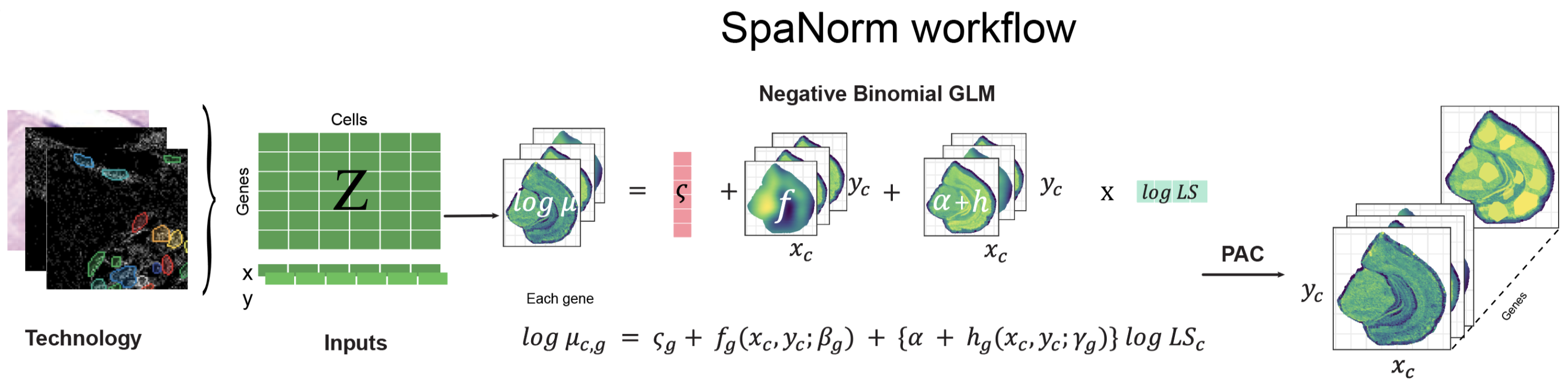
SpaNorm uses a unique approach to spatially constraint modelling approach to model gene expression (e.g., counts) and remove library size effects, while retaining biology. It achieves this through three key innovations:
- Optmial decomposition of spatial variation into spatially smooth library size associated (technical) and library size independent (biology) variation using generalized linear models (GLMs).
- Computing spatially smooth functions (using thin plate splines) to represent the gene- and location-/cell-/spot- specific size factors.
- Adjustment of data using percentile adjusted counts (PAC) (Salim et al. 2022), as well as other adjustment approaches (e.g., Pearson).
The SpaNorm package can be installed as follows:
if (!requireNamespace("BiocManager", quietly = TRUE))
    install.packages("BiocManager")

# release version
BiocManager::install("SpaNorm")
# development version from GitHub
BiocManager::install("bhuvad/SpaNorm")
Load count data
We begin by loading some example 10x Visium data profiling the
dorsolateral prefrontal cortex (DLPFC) of the human brain. The data has
~4,000 spots and covers genome-wide measurements. The example data here
is filtered to remove lowly expressed genes (using
filterGenes(HumanDLPFC, prop = 0.1)). This filtering
retains genes that are expressed in at least 10% of cells.
library(SpaNorm)
library(SpatialExperiment)
library(ggplot2)

# load sample data
data(HumanDLPFC)
# change gene IDs to gene names
rownames(HumanDLPFC) = rowData(HumanDLPFC)$gene_name
HumanDLPFC
#> class: SpatialExperiment
#> dim: 5076 4015
#> metadata(0):
#> assays(1): counts
#> rownames(5076): NOC2L HES4 ... MT-CYB AC007325.4
#> rowData names(2): gene_name gene_biotype
#> colnames(4015): AAACAAGTATCTCCCA-1 AAACACCAATAACTGC-1 ...
#>   TTGTTTCCATACAACT-1 TTGTTTGTGTAAATTC-1
#> colData names(3): cell_count sample_id AnnotatedCluster
#> reducedDimNames(0):
#> mainExpName: NULL
#> altExpNames(0):
#> spatialCoords names(2) : pxl_col_in_fullres pxl_row_in_fullres
#> imgData names(4): sample_id image_id data scaleFactor

# plot regions
p_region = plotSpatial(HumanDLPFC, colour = AnnotatedCluster, size = 0.5) +
  scale_colour_brewer(palette = "Paired", guide = guide_legend(override.aes = list(shape = 15, size = 5))) +
  ggtitle("Region")
p_region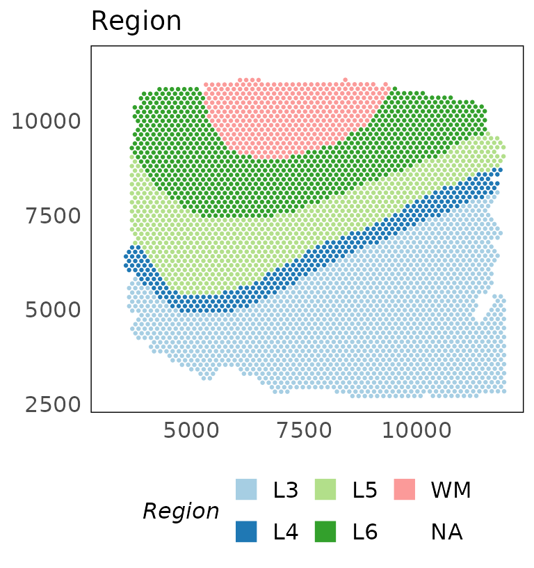
The filterGenes function returns a logical vector
indicating which genes should be kept.
# filter genes expressed in 20% of spots
keep = filterGenes(HumanDLPFC, 0.2)
table(keep)
#> keep
#> FALSE  TRUE
#>  2568  2508
# subset genes
HumanDLPFC = HumanDLPFC[keep, ]
The log-transformed raw counts are visualised below for the gene MOBP which is a marker of oligodendrocytes enriched in the white matter (WM) (Maynard et al. 2021). Despite being a marker of this region, we see that it is in fact absent from the white matter region.
logcounts(HumanDLPFC) = log2(counts(HumanDLPFC) + 1)

p_counts = plotSpatial(
    HumanDLPFC,
    colour = MOBP,
    what = "expression",
    assay = "logcounts",
    size = 0.5
  ) +
  scale_colour_viridis_c(option = "F") +
  ggtitle("logCounts")
p_region + p_counts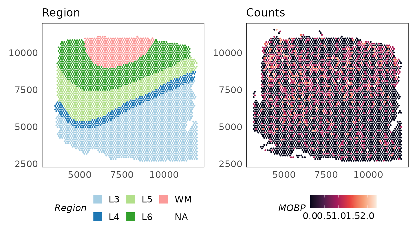
Normalise count data
SpaNorm normalises data in two steps: (1) fitting the SpaNorm model
of library sizes; (2) adjusting data using the fit model. A single call
to the SpaNorm() function is enough to run these two steps.
To speed up computation, the model is fit using a smaller proportion of
spots/cells (default is 0.25). The can be modified using the
sample.p parameter.
set.seed(36)
HumanDLPFC = SpaNorm(HumanDLPFC)
#> (1/2) Fitting SpaNorm model
#> 1004 cells/spots sampled to fit model
#> iter:  1, estimating gene-wise dispersion
#> iter:  1, log-likelihood: -3185991.766198
#> iter:  1, fitting NB model
#> iter:  1, iter:  1, log-likelihood: -3185991.766198
#> iter:  1, iter:  2, log-likelihood: -2582103.888695
#> iter:  1, iter:  3, log-likelihood: -2463315.785705
#> iter:  1, iter:  4, log-likelihood: -2425458.605075
#> iter:  1, iter:  5, log-likelihood: -2411619.260732
#> iter:  1, iter:  6, log-likelihood: -2407711.960028
#> iter:  1, iter:  7, log-likelihood: -2406494.322919
#> iter:  1, iter:  8, log-likelihood: -2406052.089545
#> iter:  1, iter:  9, log-likelihood: -2405875.012540 (converged)
#> iter:  2, estimating gene-wise dispersion
#> iter:  2, log-likelihood: -2402618.503945
#> iter:  2, fitting NB model
#> iter:  2, iter:  1, log-likelihood: -2402618.503945
#> iter:  2, iter:  2, log-likelihood: -2401826.557195
#> iter:  2, iter:  3, log-likelihood: -2401754.435364 (converged)
#> iter:  3, estimating gene-wise dispersion
#> iter:  3, log-likelihood: -2401744.259596
#> iter:  3, fitting NB model
#> iter:  3, iter:  1, log-likelihood: -2401744.259596
#> iter:  3, iter:  2, log-likelihood: -2401695.995571
#> iter:  3, iter:  3, log-likelihood: -2401686.415779 (converged)
#> iter:  4, log-likelihood: -2401686.415779 (converged)
#> (2/2) Normalising data
HumanDLPFC
#> class: SpatialExperiment
#> dim: 2508 4015
#> metadata(1): SpaNorm
#> assays(2): counts logcounts
#> rownames(2508): ISG15 SDF4 ... MT-ND6 MT-CYB
#> rowData names(2): gene_name gene_biotype
#> colnames(4015): AAACAAGTATCTCCCA-1 AAACACCAATAACTGC-1 ...
#>   TTGTTTCCATACAACT-1 TTGTTTGTGTAAATTC-1
#> colData names(3): cell_count sample_id AnnotatedCluster
#> reducedDimNames(0):
#> mainExpName: NULL
#> altExpNames(0):
#> spatialCoords names(2) : pxl_col_in_fullres pxl_row_in_fullres
#> imgData names(4): sample_id image_id data scaleFactor
The above output (which can be switched off by setting
verbose = FALSE), shows the two steps of normalisation. In
the model fitting step, 1004 cells/spots are used to fit the negative
binomial (NB) model. Subsequent output shows that this fit is performed
by alternating between estimation of the dispersion parameter and
estimation of the NB parameters by fixing the dispersion. The output
also shows that each intermediate fit converges, and so does the final
fit. The accuracy of the fit can be controlled by modifying the
tolerance parameter tol (default 1e-4).
Next, data is adjusted using the fit model. The following approaches are implemented for count data:
-
adj.method = "logpac"(default) - percentile adjusted counts (PAC) which estimates the count for each gene at each location/spot/cell using a model that does not contain unwanted effects such as the library size. -
adj.method = "person"- Pearson residuals from factoring out unwanted effects. -
adj.method = "meanbio"- the mean of each gene at each location estimated from the biological component of the model. -
adj.method = "medbio"- the median of each gene at each location estimated from the biological component of the model.
These data are stored in the logcounts assay of the
SpatialExperiment object. After normalisation, we see that MOBP is
enriched in the white matter.
p_logpac = plotSpatial(
    HumanDLPFC,
    colour = MOBP,
    what = "expression",
    assay = "logcounts",
    size = 0.5
  ) +
  scale_colour_viridis_c(option = "F") +
  ggtitle("logPAC")
p_region + p_logpac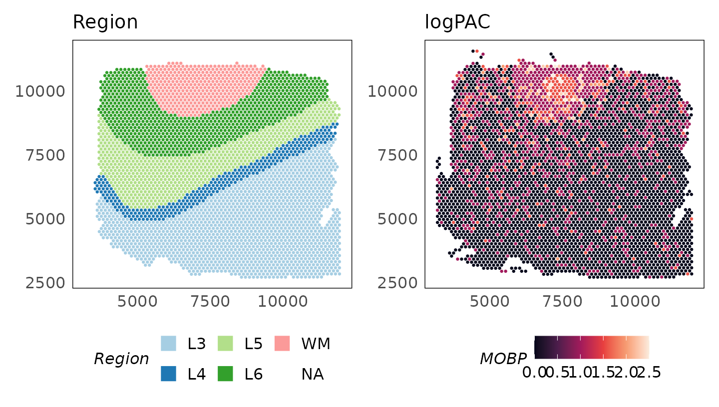
Scaling to large datasets
For large datasets, the normalisation step can be parallelised across
workers using the BPPARAM argument, which accepts any
BiocParallelParam object from the BiocParallel
package. Normalisation runs serially by default
(SerialParam()).
library(BiocParallel)
# parallelise normalisation across 4 workers
HumanDLPFC = SpaNorm(HumanDLPFC, BPPARAM = MulticoreParam(workers = 4))
When the counts assay is a DelayedArray (for example, a
disk-backed HDF5Array), SpaNorm automatically normalises
the data in blocks so that the full matrix is never loaded into memory
at once. This is detected from the data and needs no additional
arguments, and the results are identical to the in-memory path.
library(HDF5Array)
# wrap the counts as a disk-backed DelayedArray
counts(HumanDLPFC) = writeHDF5Array(counts(HumanDLPFC))
# normalisation now runs block-wise, bounding peak memory
HumanDLPFC = SpaNorm(HumanDLPFC)
When combining the two, prefer BiocParallel::SnowParam()
over MulticoreParam() for a disk-backed (e.g. HDF5-backed)
DelayedArray: fork-based workers
(MulticoreParam, the default on Linux/macOS) each inherit a
copy of the same open file handle, which can cause
HDF5Array reads from concurrent forked workers to fail or
return incorrect data.
Using Seurat objects
Users may prefer to work with Seurat. Below we convert the
SpatialExperiment object to Seurat (v5) and add spatial
coordinates extracted from the original SpatialExperiment.
The SpaNorm function can then be run directly on the Seurat object. Note
that the counts assay is used to store raw counts and the
data assay is used to store normalised values, following
Seurat conventions. SpaNorm searches for coordinates in the
images slot which contains the coordinates
slot. If not found, it will also search meta.data slot of
the Seurat object with names x and y, or with
names imagecol and imagerow. This is the order
of the search of coordinates
library(Seurat)

# create a Seurat object with the data
seurat_obj = HumanDLPFC
logcounts(seurat_obj) = counts(seurat_obj)
seurat_obj = suppressWarnings(Seurat::as.Seurat(seurat_obj))
# add spatial coordinates to Seurat meta.data from SpatialExperiment
coords = SpatialExperiment::spatialCoords(HumanDLPFC)
seurat_obj@meta.data$x = coords[, 1]
seurat_obj@meta.data$y = coords[, 2]

# run SpaNorm on Seurat (CPU backend)
seurat_obj <- SpaNorm(seurat_obj, sample.p = 0.1, df.tps = 2, backend = "cpu", verbose = TRUE)
seurat_obj
#> An object of class Seurat
#> 2508 features across 4015 samples within 1 assay
#> Active assay: originalexp (2508 features, 0 variable features)
#>  2 layers present: counts, data
Computing alternative adjustments using a precomputed SpaNorm fit
As no appropriate slot exists for storing model parameters, we currently save them in the metadata slot with the name “SpaNorm”. This also means that subsetting features (i.e., genes) or observations (i.e., cells/spots/loci) does not subset the model. In such an instance, the SpaNorm function will realise that the model no longer matches the data and re-estimates when called. If instead the model is valid for the data, the existing fit is extracted and reused.
The fit can be manually retrieved as below for users wishing to reuse
the model outside the SpaNorm framework. Otherwise, calling
SpaNorm() on an object containing the fit will
automatically use it.
# manually retrieve model
fit.spanorm = metadata(HumanDLPFC)$SpaNorm
fit.spanorm
#> SpaNormFit
#> Data: 2508 genes, 4015 cells/spots
#> Gene model: nb
#> Degrees of freedom for TPS (y,x): Biology (6,6), LS (3,3)
#> Spots/cells sampled: 25%
#> Regularisation parameter: Biology (1e-04), LS (1e-04)
#> Batch:  NULL
#> log-likelihood (per-iteration):  num [1:3] -2405875 -2401754 -2401686
#> W:  num [1:4015, 1:46] 0.2645 0.4736 0.0547 -0.1756 0.6039 ...
#> W:  - attr(*, "dimnames")=List of 2
#> W:   ..$ : chr [1:4015] "1" "2" "3" "4" ...
#> W:   ..$ : chr [1:46] "logLS" "bs.xy.bio1" "bs.xy.bio2" "bs.xy.bio3" ...
#> alpha:  num [1:2508, 1:46] 0.989 0.989 0.989 0.989 0.989 ...
#> gmean:  num [1:2508] -1.307 -1.193 -1.275 -1.445 -0.399 ...
#> psi:  num [1:2508] 0.0399 0.0409 0.04 0.0385 0.0348 ...
#> wtype:  Factor w/ 3 levels "batch","biology",..: 3 2 2 2 2 2 2 2 2 2 ...
#> sampling: all (4015), glm (1004), dispersion (500)
When a valid fit exists in the object, only the adjustment step is
performed. The model is recomputed if overwrite = TRUE or
any of the following parameters change: degrees of freedom
(df.tps), penalty parameters(lambda.a), object
dimensions, or batch specification. Alternative adjustments
can be computed as below and stored to the logcounts
assay.
# Pearson residuals
HumanDLPFC = SpaNorm(HumanDLPFC, adj.method = "pearson")
p_pearson = plotSpatial(
    HumanDLPFC,
    colour = MOBP,
    what = "expression",
    assay = "logcounts",
    size = 0.5
  ) +
  scale_colour_viridis_c(option = "F") +
  ggtitle("Pearson")

# meanbio residuals
HumanDLPFC = SpaNorm(HumanDLPFC, adj.method = "meanbio")
p_meanbio = plotSpatial(
    HumanDLPFC,
    colour = MOBP,
    what = "expression",
    assay = "logcounts",
    size = 0.5
  ) +
  scale_colour_viridis_c(option = "F") +
  ggtitle("Mean biology")

# meanbio residuals
HumanDLPFC = SpaNorm(HumanDLPFC, adj.method = "medbio")
p_medbio = plotSpatial(
    HumanDLPFC,
    colour = MOBP,
    what = "expression",
    assay = "logcounts",
    size = 0.5
  ) +
  scale_colour_viridis_c(option = "F") +
  ggtitle("Median biology")

p_region + p_counts + p_logpac + p_pearson + p_meanbio + p_medbio + plot_layout(ncol = 3)
The mean biology adjustment shows a significant enrichment of the MOBP gene in the white matter. As the overall counts of this gene are low in this sample, other methods show less discriminative power.
Varying model complexity
The complexity of the spatial smoothing function is determined by the
df.tps parameter where larger values result in more
complicated functions (default 6).
# df.tps = 2
HumanDLPFC_df2 = SpaNorm(HumanDLPFC, df.tps = 2)
p_logpac_2 = plotSpatial(
    HumanDLPFC,
    colour = MOBP,
    what = "expression",
    assay = "logcounts",
    size = 0.5
  ) +
  scale_colour_viridis_c(option = "F") +
  ggtitle("logPAC (df.tps = 2)")

# df.tps = 6 (default)
p_logpac_6 = p_logpac +
  ggtitle("logPAC (df.tps = 6)")

p_logpac_2 + p_logpac_6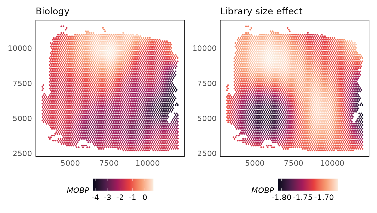
Enhancing signal
As the counts for the MOBP gene are very low, we see artifacts in the adjusted counts. As we have a model for the genes, we can increase the signal by adjusting all means by a constant factor. Applying a scale factor of 4 shows how the adjusted data are more continuous, with significant enrichment in the white matter.
# scale.factor = 1 (default)
HumanDLPFC = SpaNorm(HumanDLPFC, scale.factor = 1)
p_logpac_sf1 = plotSpatial(
    HumanDLPFC,
    colour = MOBP,
    what = "expression",
    assay = "logcounts",
    size = 0.5
  ) +
  scale_colour_viridis_c(option = "F") +
  ggtitle("logPAC (scale.factor = 1)")

# scale.factor = 4
HumanDLPFC = SpaNorm(HumanDLPFC, scale.factor = 4)
p_logpac_sf4 = plotSpatial(
    HumanDLPFC,
    colour = MOBP,
    what = "expression",
    assay = "logcounts",
    size = 0.5
  ) +
  scale_colour_viridis_c(option = "F") +
  ggtitle("logPAC (scale.factor = 4)")

p_logpac_sf1 + p_logpac_sf4 + plot_layout(ncol = 2)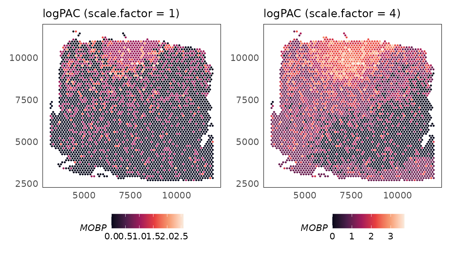
Exploring learnt functions
The plotCovariate() function can be used to explore the
learnt functions. We could study what the model has learnt about the
biology and library size effects of the MOBP gene.
p1 = plotCovariate(HumanDLPFC, colour = MOBP, covariate = "biology") +
  scale_colour_viridis_c(option = "F") +
  ggtitle("Biology")
p2 = plotCovariate(HumanDLPFC, colour = MOBP, covariate = "ls") +
  scale_colour_viridis_c(option = "F") +
  ggtitle("Library size effect")
p1 + p2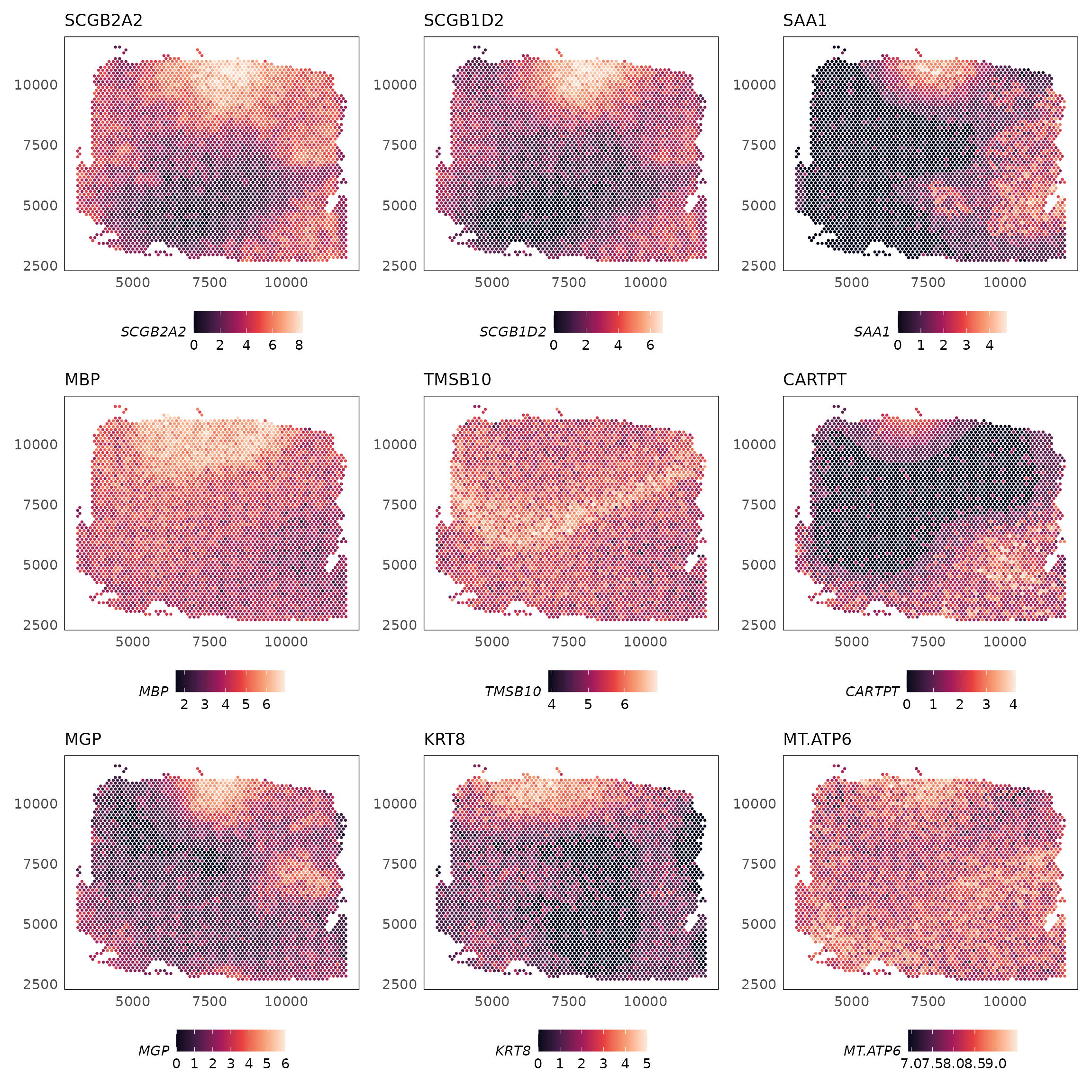
Identifying spatially variable genes
The SpaNormSVG() function can be used to identify
spatially variable genes (SVGs) in the data. This function fits a nested
model without the biological function of the form:
where is the mean of gene at location , is the log-mean of gene , is a smooth function of the spatial coordinates and representing the library size effect, and is the log-mean of the library size.
The SpaNormSVG() function fits this model and then uses
an F-test to identify spatially variable genes (SVGs).
HumanDLPFC = SpaNormSVG(HumanDLPFC)
#> (1/3) Retrieving SpaNorm model
#> (2/3) Fitting Null SpaNorm model
#> 1004 cells/spots sampled to fit model
#> iter:  1, estimating gene-wise dispersion
#> iter:  1, log-likelihood: -3190091.179683
#> iter:  1, fitting NB model
#> iter:  1, iter:  1, log-likelihood: -3190091.179683
#> iter:  1, iter:  2, log-likelihood: -2602274.983533
#> iter:  1, iter:  3, log-likelihood: -2480404.997107
#> iter:  1, iter:  4, log-likelihood: -2453594.180755
#> iter:  1, iter:  5, log-likelihood: -2450631.224623
#> iter:  1, iter:  6, log-likelihood: -2450483.720559 (converged)
#> iter:  2, estimating gene-wise dispersion
#> iter:  2, log-likelihood: -2449692.278328
#> iter:  2, fitting NB model
#> iter:  2, iter:  1, log-likelihood: -2449692.278328
#> iter:  2, iter:  1, log-likelihood: -2449692.278328
#> iter:  2, iter:  1, log-likelihood: -2449692.278328
#> iter:  2, iter:  2, log-likelihood: -2449692.278328
#> iter:  2, iter:  2, log-likelihood: -2449692.278328
#> iter:  2, iter:  2, log-likelihood: -2449692.278328
#> iter:  2, iter:  3, log-likelihood: -2449692.278328 (converged)
#> iter:  3, estimating gene-wise dispersion
#> iter:  3, log-likelihood: -2449692.278328
#> iter:  3, fitting NB model
#> iter:  3, iter:  1, log-likelihood: -2449692.278328
#> iter:  3, iter:  1, log-likelihood: -2449692.278328
#> iter:  3, iter:  1, log-likelihood: -2449692.278328
#> iter:  3, iter:  2, log-likelihood: -2449692.278328
#> iter:  3, iter:  2, log-likelihood: -2449692.278328
#> iter:  3, iter:  2, log-likelihood: -2449692.278328
#> iter:  3, iter:  3, log-likelihood: -2449692.278328 (converged)
#> iter:  4, log-likelihood: -2449692.278328 (converged)
#> (3/3) Finding SVGs
#> 253 SVGs found (FDR < 0.05)
HumanDLPFC
#> class: SpatialExperiment
#> dim: 2508 4015
#> metadata(2): SpaNorm SpaNormNull
#> assays(2): counts logcounts
#> rownames(2508): ISG15 SDF4 ... MT-ND6 MT-CYB
#> rowData names(5): gene_name gene_biotype svg.F svg.p svg.fdr
#> colnames(4015): AAACAAGTATCTCCCA-1 AAACACCAATAACTGC-1 ...
#>   TTGTTTCCATACAACT-1 TTGTTTGTGTAAATTC-1
#> colData names(3): cell_count sample_id AnnotatedCluster
#> reducedDimNames(0):
#> mainExpName: NULL
#> altExpNames(0):
#> spatialCoords names(2) : pxl_col_in_fullres pxl_row_in_fullres
#> imgData names(4): sample_id image_id data scaleFactor
The topSVGs() function can be used to retrieve the top
spatially variable genes (SVGs) at a given false discovery rate (FDR).
These are stored in the rowData slot of the
SpatialExperiment object.
svgs = topSVGs(HumanDLPFC, n = 10)
svgs
#>            svg.F         svg.p       svg.fdr
#> SCGB2A2 94.52335  0.000000e+00  0.000000e+00
#> SCGB1D2 52.79914 9.543647e-305 1.196773e-301
#> SAA1    38.89095 1.684880e-229 1.408560e-226
#> MBP     30.30317 8.683568e-180 5.444597e-177
#> TMSB10  26.85346 4.454734e-159 2.234495e-156
#> CARTPT  25.20582 4.917004e-149 2.055308e-146
#> MGP     24.98233 1.152100e-147 4.127810e-145
#> MT-ATP6 21.35937 3.256268e-125 1.020840e-122
#> MT-CO2  21.32369 5.446460e-125 1.517747e-122
#> HPCAL1  20.93350 1.519761e-122 3.465055e-120
We can visualise the spatially variable genes using the
plotSpatial() function.
# fix gene names
rownames(HumanDLPFC) = gsub("-", ".", rownames(HumanDLPFC))
rownames(svgs) = gsub("-", ".", rownames(svgs))

lapply(rownames(svgs)[1:9], function(g) {
  plotSpatial(HumanDLPFC, colour = !!sym(g), what = "expression", assay = "logcounts", size = 0.5) +
    scale_colour_viridis_c(option = "F") +
    ggtitle(g) +
    theme(legend.position = "bottom")
}) |>
  wrap_plots(ncol = 3)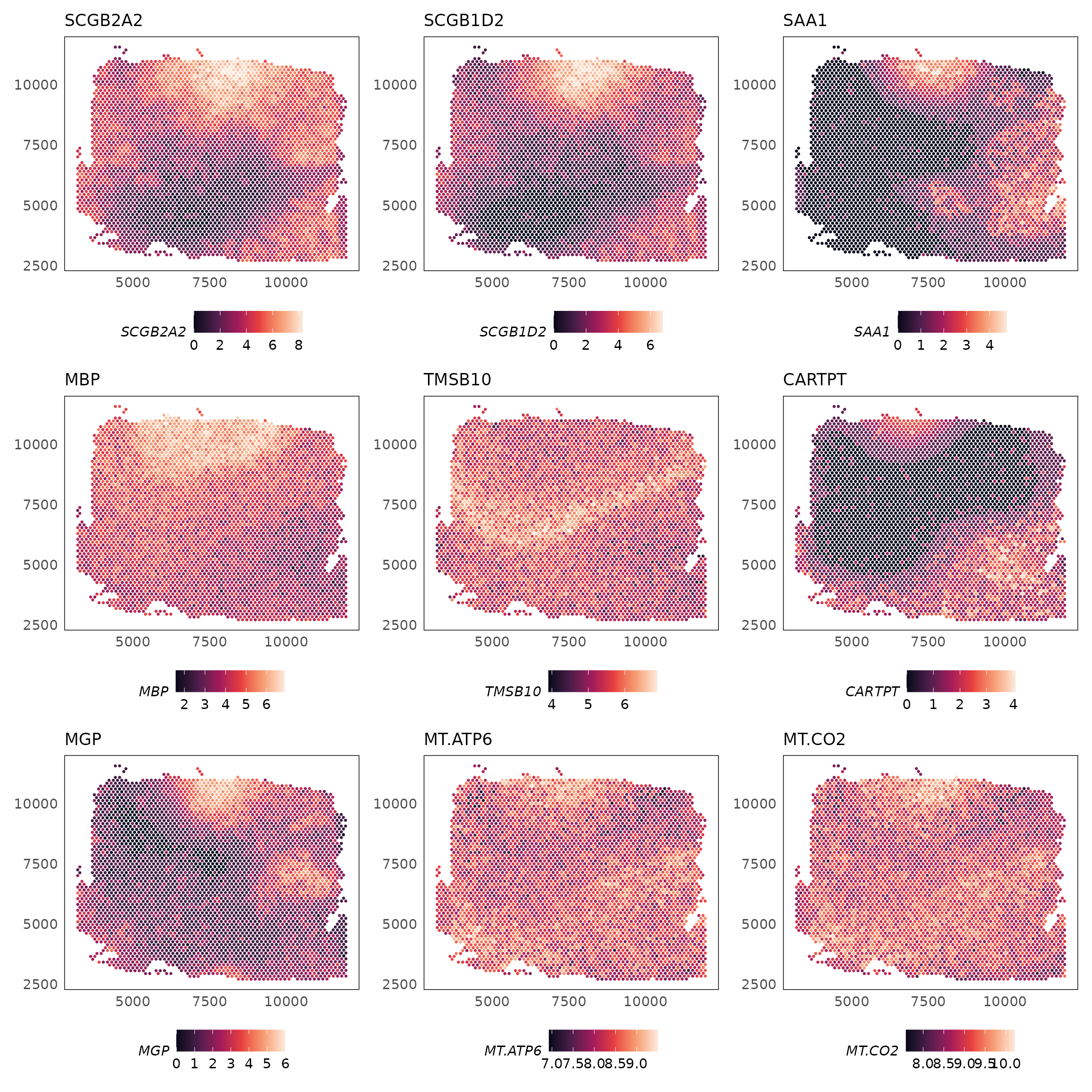
GLM-PCA
PCA on log-transfomed counts has been show to distort low dimensional
features in single-cell datasets (Townes et al.
2019). As spatial transcriptomics data follows similar
distributions, this is also the case for spatial transcriptomics data.
GLM-PCA which computes PCA directly on the counts is a better approach
to perform PCA on spatial transcriptomics data. While the GLM-PCA
algorithm itself is computationally intensive, an approximation proposed
in the original manuscripts is to fit a null model to the data and
perform PCA on the deviance or Pearson residuals. This null model is the
one fit above to estimate SVGs. SpaNorm implements the GLM-PCA
approximation using the SpaNormPCA() function. Users can
specify the features to use from the SVG calling, using cutoffs for the
top SVGs to use (recommended) or using a FDR cutoff. The interface to
this function is similar to the scater::runPCA() function
and the results are stored in the reducedDim slot of the
SpatialExperiment object using the proposed name (default is “PCA”).
This function should always be run calling SVGs
(SpaNormSVG()) first.
library(scater)

HumanDLPFC = SpaNormPCA(HumanDLPFC, ncomponents = 50, svg.fdr = 0.2, nsvgs = Inf)
HumanDLPFC = runUMAP(HumanDLPFC, n_neighbors = 20, min_dist = 0.3)
plotUMAP(HumanDLPFC, colour_by = "AnnotatedCluster", size_by = "cell_count") +
  scale_colour_brewer(palette = "Paired", guide = guide_legend(override.aes = list(shape = 15, size = 5))) +
  labs(title = "UMAP derived from SpaNorm PCA", colour = "Cluster")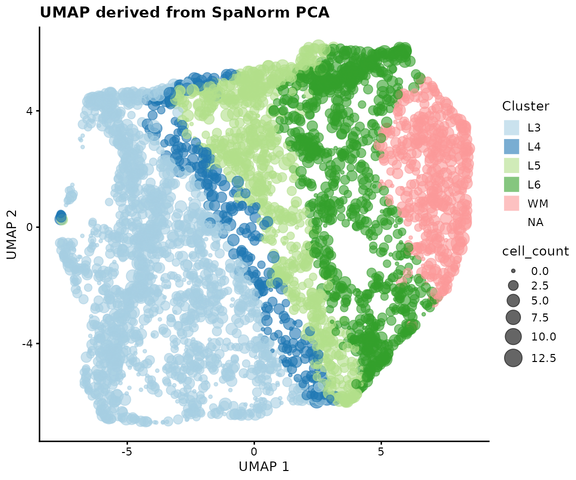
Fitting a custom model
SpaNorm’s underlying negative binomial fitting engine is also
available as a standalone, general-purpose per-gene GLM fitter via
fitNB(). This is useful for packages that want SpaNorm’s
IRLS fitting machinery (per-gene dispersion estimation, ridge
regularisation, robust winsorisation) over their own design matrix,
rather than SpaNorm’s spatial (library-size/biology) model. Unlike
SpaNorm(), fitNB() fits
log(mu) = W %*% t(alpha) directly, with no built-in
intercept – include a column of ones in W if a per-gene
baseline is required.
Session information
sessionInfo()
#> R version 4.6.1 (2026-06-24)
#> Platform: x86_64-pc-linux-gnu
#> Running under: Ubuntu 24.04.4 LTS
#>
#> Matrix products: default
#> BLAS:   /usr/lib/x86_64-linux-gnu/openblas-pthread/libblas.so.3
#> LAPACK: /usr/lib/x86_64-linux-gnu/openblas-pthread/libopenblasp-r0.3.26.so;  LAPACK version 3.12.0
#>
#> locale:
#>  [1] LC_CTYPE=C.UTF-8       LC_NUMERIC=C           LC_TIME=C.UTF-8
#>  [4] LC_COLLATE=C.UTF-8     LC_MONETARY=C.UTF-8    LC_MESSAGES=C.UTF-8
#>  [7] LC_PAPER=C.UTF-8       LC_NAME=C              LC_ADDRESS=C
#> [10] LC_TELEPHONE=C         LC_MEASUREMENT=C.UTF-8 LC_IDENTIFICATION=C
#>
#> time zone: UTC
#> tzcode source: system (glibc)
#>
#> attached base packages:
#> [1] stats4    stats     graphics  grDevices utils     datasets  methods
#> [8] base
#>
#> other attached packages:
#>  [1] Seurat_5.5.1                SeuratObject_5.4.0
#>  [3] sp_2.2-1                    scater_1.40.2
#>  [5] scuttle_1.22.0              SpatialExperiment_1.22.0
#>  [7] SingleCellExperiment_1.34.0 SummarizedExperiment_1.42.0
#>  [9] Biobase_2.72.0              GenomicRanges_1.64.0
#> [11] Seqinfo_1.2.0               IRanges_2.46.0
#> [13] S4Vectors_0.50.1            BiocGenerics_0.58.1
#> [15] generics_0.1.4              MatrixGenerics_1.24.0
#> [17] matrixStats_1.5.0           patchwork_1.3.2
#> [19] ggplot2_4.0.3               SpaNorm_1.7.4
#>
#> loaded via a namespace (and not attached):
#>   [1] RcppAnnoy_0.0.23       splines_4.6.1          later_1.4.8
#>   [4] tibble_3.3.1           polyclip_1.10-7        fastDummies_1.7.6
#>   [7] lifecycle_1.0.5        edgeR_4.10.1           globals_0.19.1
#>  [10] processx_3.9.0         lattice_0.22-9         MASS_7.3-65
#>  [13] magrittr_2.0.5         limma_3.68.4           plotly_4.12.0
#>  [16] sass_0.4.10            rmarkdown_2.31         jquerylib_0.1.4
#>  [19] yaml_2.3.12            metapod_1.20.0         httpuv_1.6.17
#>  [22] otel_0.2.0             sctransform_0.4.3      spam_2.11-4
#>  [25] spatstat.sparse_3.2-0  reticulate_1.46.0      cowplot_1.2.0
#>  [28] pbapply_1.7-4          RColorBrewer_1.1-3     abind_1.4-8
#>  [31] Rtsne_0.17             purrr_1.2.2            coro_1.1.0
#>  [34] torch_0.17.0           ggrepel_0.9.8          irlba_2.3.7
#>  [37] spatstat.utils_3.2-3   listenv_1.0.0          BiocStyle_2.40.0
#>  [40] goftest_1.2-3          RSpectra_0.16-2        spatstat.random_3.5-0
#>  [43] dqrng_0.4.1            fitdistrplus_1.2-6     parallelly_1.48.0
#>  [46] pkgdown_2.2.1          codetools_0.2-20       DelayedArray_0.38.2
#>  [49] prettydoc_0.4.1        tidyselect_1.2.1       farver_2.1.2
#>  [52] ScaledMatrix_1.20.0    viridis_0.6.5          spatstat.explore_3.8-1
#>  [55] jsonlite_2.0.0         BiocNeighbors_2.6.0    progressr_1.0.0
#>  [58] ggridges_0.5.7         survival_3.8-6         systemfonts_1.3.2
#>  [61] tools_4.6.1            ragg_1.5.2             ica_1.0-3
#>  [64] Rcpp_1.1.2             glue_1.8.1             gridExtra_2.3.1
#>  [67] SparseArray_1.12.2     xfun_0.60              dplyr_1.2.1
#>  [70] withr_3.0.3            BiocManager_1.30.27    fastmap_1.2.0
#>  [73] bluster_1.22.0         callr_3.8.0            digest_0.6.39
#>  [76] rsvd_1.0.5             R6_2.6.1               mime_0.13
#>  [79] textshaping_1.0.5      scattermore_1.2        tensor_1.5.1
#>  [82] spatstat.data_3.1-9    tidyr_1.3.2            data.table_1.18.4
#>  [85] FNN_1.1.4.1            httr_1.4.8             htmlwidgets_1.6.4
#>  [88] S4Arrays_1.12.0        uwot_0.2.4             pkgconfig_2.0.3
#>  [91] gtable_0.3.6           lmtest_0.9-40          S7_0.2.2
#>  [94] XVector_0.52.0         htmltools_0.5.9        dotCall64_1.2
#>  [97] scales_1.4.0           png_0.1-9              spatstat.univar_3.2-0
#> [100] scran_1.40.0           knitr_1.51             reshape2_1.4.5
#> [103] rjson_0.2.23           nlme_3.1-169           cachem_1.1.0
#> [106] zoo_1.8-15             stringr_1.6.0          KernSmooth_2.23-26
#> [109] parallel_4.6.1         miniUI_0.1.2           vipor_0.4.7
#> [112] desc_1.4.3             pillar_1.11.1          grid_4.6.1
#> [115] vctrs_0.7.3            RANN_2.6.2             promises_1.5.0
#> [118] BiocSingular_1.28.0    beachmat_2.28.0        xtable_1.8-8
#> [121] cluster_2.1.8.2        beeswarm_0.4.0         evaluate_1.0.5
#> [124] magick_2.9.1           cli_3.6.6              locfit_1.5-9.12
#> [127] compiler_4.6.1         rlang_1.3.0            future.apply_1.20.2
#> [130] labeling_0.4.3         ps_1.9.3               plyr_1.8.9
#> [133] fs_2.1.0               ggbeeswarm_0.7.3       stringi_1.8.7
#> [136] deldir_2.0-4           viridisLite_0.4.3      BiocParallel_1.46.0
#> [139] lazyeval_0.2.3         spatstat.geom_3.8-1    Matrix_1.7-5
#> [142] RcppHNSW_0.7.0         bit64_4.8.2            future_1.70.0
#> [145] statmod_1.5.2          shiny_1.14.0           ROCR_1.0-12
#> [148] igraph_2.3.3           bslib_0.11.0           bit_4.6.0