Part II: Identify cell states using PhiSpace
Jiadong Mao
Melbourne Integrative Genomics (MIG), The University of Melbournejiadong.mao@unimelb.edu.au
Yifan Qin
Melbourne Integrative Genomics (MIG), The University of Melbourneyifan.qin.1@unimelb.edu.au
Nov 2025
Source:vignettes/Part_II_PhiSpace.Rmd
Part_II_PhiSpace.RmdAcronyms
ST: spatial transcriptomics
sc: single-cell
sce: SingleCellExperiment
spe: SpatialExperiment
NSCLC: non-small cell lung cancer
H&E: hematoxylin and eosin (staining)
EMT: epithelial-to-mesenchymal transition
PLS: partial least squares
CAF: cancer-associated fibroblast
TLS: tertiary lymphoid structure
LUAD: lung ardenocarcinoma (a type of NSCLC)
LUSC: lung squamous cell carcinoma (a type of NSCLC)
What’s covered in Part II
Background: mixture of cell identity in ST studies
Characterising cell states is an important component of spatial omics studies. By cell states we mean transcriptional programs of cells at the time of sequencing, which provides a snapshot of what the cells are doing. Cell state characterisation goes beyond individual marker genes and look at transcriptional programs, and is essential for a more interpretable biological story: instead of saying ‘gene A promotes gene B’s function’, cell state characterisation allows us to say things like ‘A type cells interacted with B type cells to promote certain function’.
A common way to characterise cell states is based on scRNA-seq reference datasets, or simply references. That is, to see what cell states there are in a tissue section, we take existing scRNA-seq datasets with well defined cell state annotations, and then transfer the cell states from sc reference to spatial query.
An immediate problem we encounter when using scRNA-seq reference to annotate ST queries is the mixture of cell identity problem in ST data. By mixture of cell identity we mean the existence of transcripts from multiple cells in a single spatial measurement unit. In scRNA-seq, the measurement unit is a single cell (after appropriate quality control); but ST lacks exact sc resolution.
This may sound a bit surprising as we often see phrases like ‘spatial single-cell sequencing’, or claims such as ‘XXX has achieved real single-cell resolution’. We only need to note that scRNA-seq obtains sc resolution via a cell isolation step, where the tissue sample is dissolved and single cells allocated to droplets or micro-wells; in ST such cell isolation step does not exist. Instead in ST we have either
- supercellular resolution, where each spatial unit is physically larger than the typical size of a cell; or
- subcellular resolution, where each spatial unit is smaller than the typical size of a cell.
We sometimes see ‘near-cellular’ ST platforms (eg Slide-seqV2). This simply means that the size of their spatial units is close to that of a cell (10μm). In this case, a spatial unit may still contain transcripts from multiple neighbouring cells.
Via imaging and machine learning techniques, ST vendors sometimes provide additional cell membrane staining for cell segmentation. That is, via based on staining information we can locate nuclei and membranes of individual cells. Then we can attribute transcripts to segmented cells. In this case indeed we can view ST data with cell segmentation as having sc resolution. But keep in mind that cell segmentation tend to suffer when the tissue has been cut too thick, or the cells are irregularly shaped (neurons and astrocytes in the brain), or simply too crowded (eg in the spleen).
In addition, phenomenon such as transcript diffusion, ie transcripts drifting to different locations during sequencing, may also cause transcripts from different cells to appear at the same spatial unit.
All these imply that mixture of cell identity will be a common phenomenon in ST data. Hence having scRNA-seq references with exact sc resolution and relatively reliable annotation is important for the deconvolution of cell states in ST studies.
What is PhiSpace
PhiSpace is a tool for identify continuous cell states in sc and spatial omics data using bulk or single-cell references. PhiSpace is specialised in dealing with mixture of cell identities due to biological (transitional and disease-altered cell states) or technical (ST sequencing as reviewed above) reasons. PhiSpace uses PLS regression (or soft classification) to model continuously predict cell states using omics features such as gene expression. This flexible framework enables PhiSpace to deal with:
multi-reference annotation, where there are multiple reference datasets to be used;
multi-omics annotation, where both reference and query contain multiple omics types (eg CITE-seq with RNA and surface protein);
bridge annotation, where the reference and query contain different omics types (eg scRNA-seq and scATAC-seq, an additional bridge dataset containing both omics is required);
large scale annotation, where both reference and query data contain a huge number of cells.
The two main references for PhiSpace, applied to single-cell multiomics studies and ST studeis, are
Mao, J., Deng, Y. and Lê Cao, K.-A. (Accepted). Φ-Space: Continuous phenotyping of single-cell multi-omics data. Genome Biology. [bioRxiv preprint]
Mao, J., Choi, J. & Lê Cao, K.-A. (2025). Φ-Space ST: a platform-agnostic method to identify cell states in spatial transcriptomics studies. bioRxiv.
Summary of Part II
In this part, we will focus on the following ways of using PhiSpace for ST data:
How to run PhiSpace;
How to use PhiSpace cell state annotations for downstream analyses such as spatial clustering; and
Multi-sample analysis.
Load packages and define some functions.
# remotes::install_github("bhuvad/CosMxSpatialAnalysisWorkshop", ref = "PhiSpace")

# Key methods
suppressPackageStartupMessages(library(PhiSpace))
suppressPackageStartupMessages(library(vizOmics)) # Sister package of PhiSpace for visualisation
suppressPackageStartupMessages(library(SpaNorm))
suppressPackageStartupMessages(library(hoodscanR))
# Plotting and publishing results
suppressPackageStartupMessages(library(ggplot2))
suppressPackageStartupMessages(library(dplyr))
suppressPackageStartupMessages(library(magrittr))
suppressPackageStartupMessages(library(ggpubr))
suppressPackageStartupMessages(library(tidyr))
suppressPackageStartupMessages(library(ComplexHeatmap))
suppressPackageStartupMessages(library(seriation))

suppressPackageStartupMessages(library(CosMxSpatialAnalysisWorkshop))

## Some parameters and functions
tissueNames_CosMx <- c(
  "Lung5_Rep1", "Lung5_Rep2", "Lung5_Rep3",
  "Lung6", "Lung9_Rep1", "Lung9_Rep2", "Lung12", "Lung13"
)
How to run PhiSpace: the basics
Make sure that you’ve installed the newest version of key packages, including PhiSpace, SpaNorm and jazzPanda, as these packages are under active maintenance and development.
Using one scRNA-seq reference
Running PhiSpace is straightforward. We need:
- A reference sce object, containing normalised gene expression and
cell phenotypes of interest (discrete or continuous) in
colData(sce); - Query spe object, containing normalised gene expression and spatial coordinates of spatial units;
- A set of genes shared between reference and query.
We’ve already seen the PhiSpace annotation of a small subsection of Lung5 from the CosMx dataset (He et al., 2022) in Part I. Now let’s see how the annotation was computed.
Load the reference and query data.
Then we normalise the gene counts in reference and query. By default,
we do a log(counts + 1) normalisation of both count matrices via
PhiSpace::logTransf. Note that this is just a log1p
transform of raw counts, not relative counts as in standard sc pipelines
such as Seurat and scanpy. This is because library sizes confound
biology in many ST datasets.
Alternatively, we also recommend trying more sophisticated normalisation methods:
Normalise sc reference by scran;
Normalise spatial query by SpaNorm.
ref_luca <- scranTransf(ref_luca)## Warning in (function (x, sizes, min.mean = NULL, positive = FALSE, scaling =
## NULL) : encountered non-positive size factor estimates
## Warning in (function (x, sizes, min.mean = NULL, positive = FALSE, scaling =
## NULL) : encountered non-positive size factor estimates
# lung5_norm already normalised by SpaNormThe column containing cell type annotations is
cell_type.
colData(ref_luca) ## DataFrame with 6745 rows and 4 columns
## patient cell_type ncells sizeFactor
## <factor> <factor> <integer> <numeric>
## 1 Adams_Kaminski_2020_001C Alveolar cell type 1 40 0.009094104
## 2 Adams_Kaminski_2020_001C Alveolar cell type 2 2 0.000554093
## 3 Adams_Kaminski_2020_001C B cell 31 0.004495114
## 4 Adams_Kaminski_2020_001C Ciliated 14 0.004371639
## 5 Adams_Kaminski_2020_001C Club 1 0.001205301
## ... ... ... ... ...
## 6741 Zilionis_Klein_2019_patient_7 cDC1 3 0.00108161
## 6742 Zilionis_Klein_2019_patient_7 cDC2 59 0.03142964
## 6743 Zilionis_Klein_2019_patient_7 myeloid dividing 6 0.00372641
## 6744 Zilionis_Klein_2019_patient_7 pDC 54 0.01363359
## 6745 Zilionis_Klein_2019_patient_7 transitional club/AT2 22 0.00925889
YtrainName <- "cell_type"PhiSpace::PhiSpace is a convenient wrapper of the PhiSpace annotation method. It can take a list of sce objects as reference and a list of spe objects as query. First let’s try PhiSpace using one reference and one query.
lung5_norm <- PhiSpace(
  reference = ref_luca, query = lung5_norm,
  phenotypes = YtrainName, refAssay = "logcounts", regMethod = "PLS"
)
reducedDim(lung5_norm, "PhiSpace")[1:5,1:5]
## Alveolar cell type 1 Alveolar cell type 2 B cell
## Lung5_Rep3_16_1 0.16924829 -0.06514877 -0.111546143
## Lung5_Rep3_16_10 -0.08610136 0.06488480 0.004723444
## Lung5_Rep3_16_100 0.09953434 0.01063588 0.287948903
## Lung5_Rep3_16_1000 -0.10631679 0.07567622 -0.144980073
## Lung5_Rep3_16_1001 0.01475941 -0.02031551 -0.185642731
## Ciliated Club
## Lung5_Rep3_16_1 -0.07360635 -0.18794040
## Lung5_Rep3_16_10 0.30635257 -0.14147385
## Lung5_Rep3_16_100 0.00328921 -0.15294138
## Lung5_Rep3_16_1000 -0.12491205 0.08877949
## Lung5_Rep3_16_1001 0.25572495 -0.28091604The first output of PhiSpace is a spatial unit by cell type matrix
deposited in reducedDim(lung5_norm, "PhiSpace"). It’s a
reducedDim object since we view cell state characterisation
as dimension reduction from the omics space to the
phenotype space. That is, after PhiSpace, the cell
state of each cell is characterised by (dozens of) cell types in the
reference, instead of expression levels of (tens of thousands of)
genes.
All our downstream analyses will be based on
reducedDim(lung5_norm, "PhiSpace"), which we simply refer
to as PhiSpace scores.
We can use PhiSpace::getClass to discretise PhiSpace
scores, so that each spatial unit gets a single cell type label
receiving the highest score compared to other cell types. Note that this
discretisation makes sense if your spatial units can be viewed as cells,
eg via cell segmentation.
lung5_norm$PhiCellType <- getClass(reducedDim(lung5_norm, "PhiSpace"))Dozens of cell types are difficult to visualise using a standard scatter plot. We could try interactive plots instead.
p <- VizSpatial(lung5_norm, ptSize = 1, groupBy = "PhiCellType")
p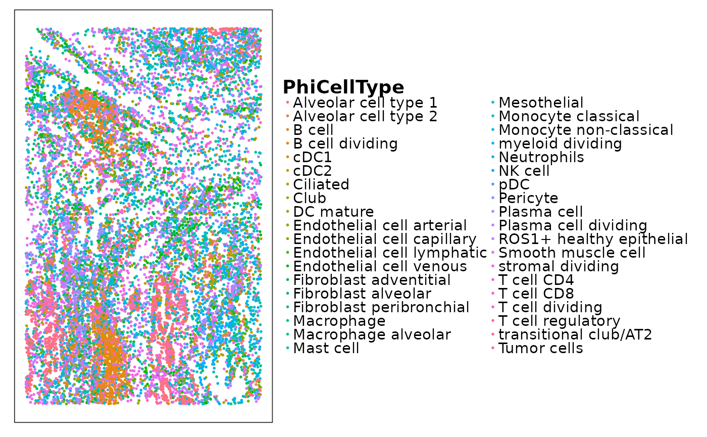
plotly::ggplotly(p)What about cases where you do not have reliable cell segmentation? Generally we do not recommend discretisation. There are many other platform-agnostic tools for analysing PhiSpace scores. For example, we can plot spatial heatmaps to show the spatial distribution of all PhiSpace scores. Often by viewing these heatmaps, we can already see a lot of intriguing biology.
Run the following code and the function will ask you to create a directory to store all heatmaps.
saveCellTypeMaps(lung5_norm, tissueName = "lung5_norm_sub", freeColScale = T, censQuant = 0.5, psize = 0.8)Now let’s look at these heatmaps. What can you see?
Multiple references?
Sometimes it might be preferable to use multiple references to annotate a single query. This could be due to
cross-validation of annotation results;
leveraging cell states defined in multiple disease systems (healthy and fibrotic lungs);
Here in addition to the Luca reference from NSCLC, we took a scRNA-seq dataset from patients with lung fibrosis (Natri et al., 2024). Although fibrotic lungs do not have cancer cells, it contains rich cell states from complex inflammatory microenvironment, which contributes to characterising cancer cell states.
Since the lung fibrosis dataset was too big. Here we provide the output, ie PhiSpace scores derived from both the Luca and the fibrosis references.
data("sc_lung5_norm_sub")
reducedDim(lung5_norm, "Phi5Ref") <- sc_lung5_norm_sub
saveCellTypeMaps(lung5_norm, tissueName = "lung5_norm_sub", methodName = "Phi5Ref", freeColScale = T, censQuant = 0.5, psize = 0.8)
More analyses based on PhiSpace scores
We’ve had some hands-on experience running PhiSpace on a small subset of Lung5. Next we will look into the PhiSpace scores and use them to discover
spatial patterns of cell types, and how they help to generate hypotheses about lung cancer;
spatial domains/niches and their differential cell states;
cell type colocalisation and how it differentiates different niches in different samples.
First we load the list of spe objects corresponding to the 8 NSCLC tissue samples. To save RAM, these spe objects only contained a 50% subsample of cells. Also they did not contain gene expression matrices, which were the most RAM-intensive part of these objects. Only metadata and pre-computed PhiSpace scores were provided.
## We splited allTissues, the list of 8 spe objects, into three parts due to GitHub file size limit
data("allTissues1")
data("allTissues2")
data("allTissues3")
allTissues <- c(allTissues1, allTissues2, allTissues3)
rm(allTissues1, allTissues2, allTissues3); gc() # Remove objects to free up RAM
## used (Mb) gc trigger (Mb) max used (Mb)
## Ncells 9635866 514.7 15940374 851.4 15940374 851.4
## Vcells 72539952 553.5 128590788 981.1 125625655 958.5Each spe object contains empty gene expression (the dimension is 1 by 43296).
allTissues[["Lung5_Rep1"]]## class: SpatialExperiment
## dim: 1 46526
## metadata(0):
## assays(1): counts
## rownames: NULL
## rowData names(0):
## colnames(46526): Lung5_Rep1_27_1218 Lung5_Rep1_16_2302 ...
## Lung5_Rep1_5_856 Lung5_Rep1_22_879
## colData names(17): sample_id cell_id ... multiSampClust BanksyClust
## reducedDimNames(1): PhiSpace
## mainExpName: NULL
## altExpNames(0):
## spatialCoords names(2) : x y
## imgData names(1): sample_idLet’s first look at the whole tissue range of Lung 5. There are three biological repeats, being consecutive tissue sections, from that lung.
If we simply plot the total RNA counts within each cell, what can we see?
VizSpatial(allTissues[["Lung5_Rep1"]], groupBy = "total", ptSize = 1, reOrder = T)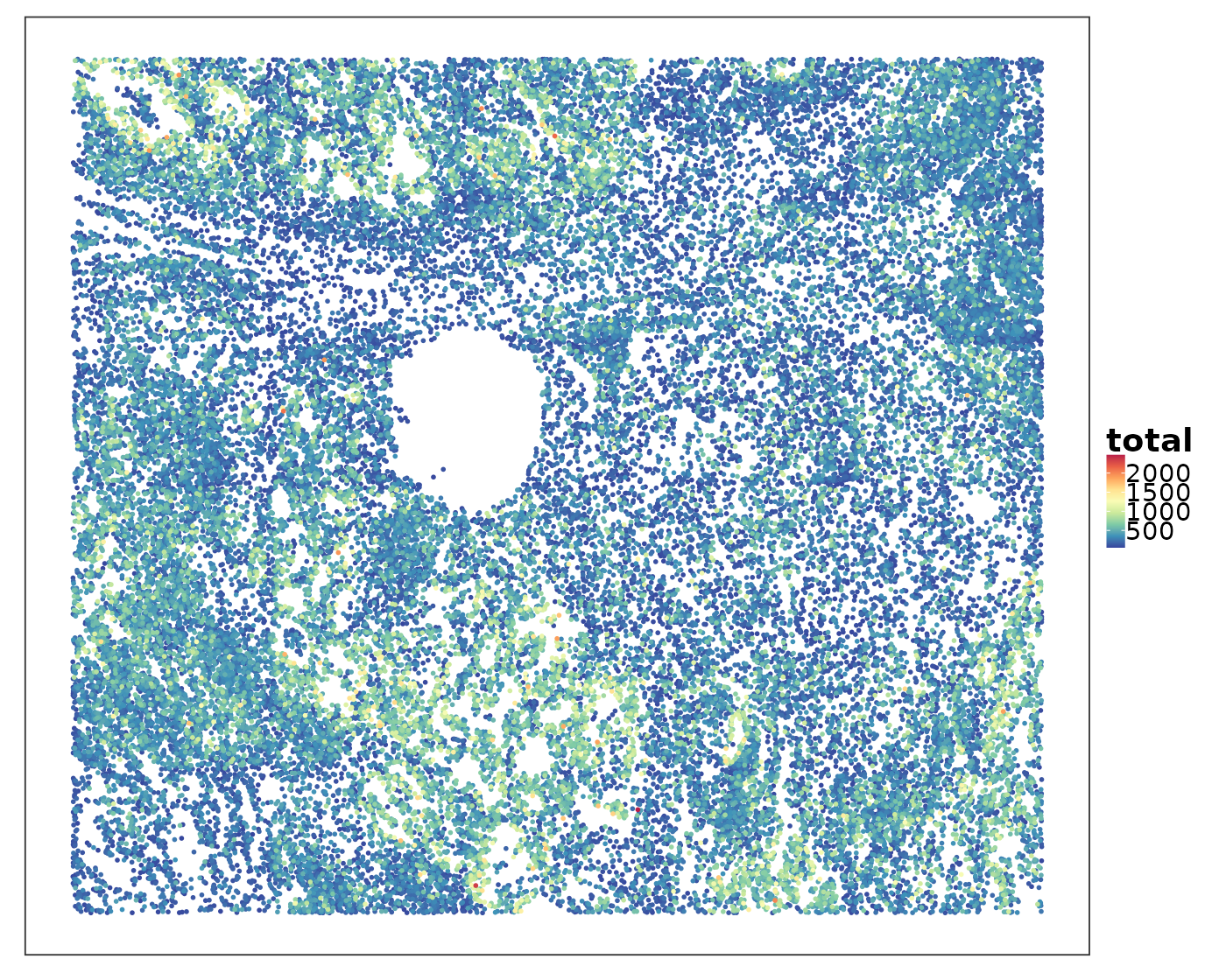
VizSpatial(allTissues[["Lung6"]], groupBy = "total", ptSize = 1, reOrder = T)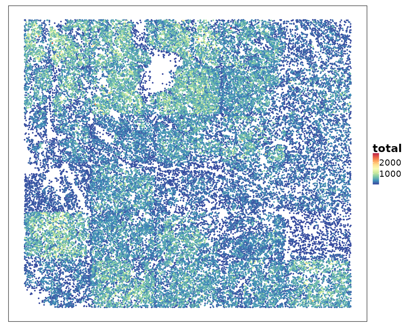
Some areas contained higher RNA content than others. Let’s visualise the spatial niches defined by a pathologist based on H&E images to find out if certain niches tended to have higher RNA content.
VizSpatial(
  allTissues[["Lung5_Rep1"]], ptSize = 0.5, groupBy = "region", legend.position = "bottom", legend.symb.size = 2
) 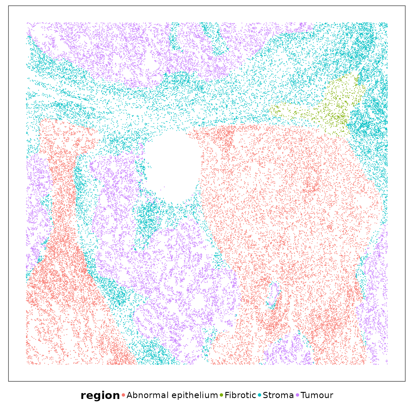
VizSpatial(
  allTissues[["Lung6"]], ptSize = 0.5, groupBy = "region", legend.position = "bottom", legend.symb.size = 2
) 
Same as before, we can save the spatial heatmaps of all cell type annotations.
saveCellTypeMaps(allTissues[["Lung5_Rep1"]], tissueName = "Lung5_Rep1", freeColScale = T, censQuant = 0.5, psize = 0.5)These spatial heatmaps are already quite revealing. Keeping the pathological niches in mind, we can have some preliminary findings:
KRT5-/KRT17+ epithelial cells are a type of abnormal epithelial cells seen in PF. There’s evidence that this type of epithelial cells can be derived from transitional AT2 cells, which are also enriched in tumour region;
Mesothelial cells shouldn’t be here – they form the outermost layer of the lungs. The presnece of this identity implies potential EMT;
gCap and aCap are two types of capillary cells with very different distributions in stroma vs abnormal stroma (capillaries are tiny blood vessels crucial for gas exchange between the alveoli and the blood).
query <- allTissues[["Lung5_Rep1"]]
# Tumour region
VizSpatial(query, ptSize = 0.8, reducedDim = "Tumour(luca)", legend.position = "bottom", censor = T)
VizSpatial(query, ptSize = 0.8, reducedDim = "KRT5-/KRT17+(epi)", legend.position = "bottom", censor = T)
VizSpatial(query, ptSize = 0.8, reducedDim = "AT2_Trans(epi)", legend.position = "bottom", censor = T)
VizSpatial(query, ptSize = 0.8, reducedDim = "Mesothelial(mesen)", legend.position = "bottom", censor = T)
# TLS
VizSpatial(query, ptSize = 0.8, reducedDim = "cDC1(immu)", legend.position = "bottom", censor = T)
VizSpatial(query, ptSize = 0.8, reducedDim = "CD4(immu)", legend.position = "bottom", censor = T)
VizSpatial(query, ptSize = 0.8, reducedDim = "B(immu)", legend.position = "bottom", censor = T)
# Stroma
VizSpatial(query, ptSize = 1, reducedDim = "Ciliated(epi)", legend.position = "bottom", censor = T)
VizSpatial(query, ptSize = 1, reducedDim = "gCap(endo)", legend.position = "bottom", censor = T)
VizSpatial(query, ptSize = 1, reducedDim = "aCap(endo)", legend.position = "bottom", censor = T)
VizSpatial(query, ptSize = 1, reducedDim = "FB_Myo(mesen)", legend.position = "bottom", censor = T)
VizSpatial(query, ptSize = 1, reducedDim = "FB_Myo_Act(mesen)", legend.position = "bottom", censor = T)
Niche identification
In spatial biology it is often desirable to identify cellular niches in tissue section. Each niche (or ‘domain’) occupies a continuous area and has a certain combination of cell states. Note that the concept of niche is very different from that of cellular clusters (or cell types): niches are required to have certain level of continuity in space, whereas a cell cluster can be scattered around in space.
Based on H&E images, a pathologist can identify niches based on morphology. But usually such niches are quite coarse-grained. Based on molecular information such as gene expression, we can identify fine-grained niches. This can be done using unsupervised clustering of gene expression profiles, using methods such as Banksy (Singhal et al., 2024).
Gene expression clustering by Bansky
How Banksy works
Banksy is a spatially-aware clustering algorithm for identifying niches. By ‘spatially-aware’ we mean methods that take into account the spatial information. Perhaps the most straightforward spatially-aware approach is spatial smoothing, which is the foundation of Banksy. Banksy augments the gene expression of each spatial unit by smoothing it using the gene expression of neighbouring units. Then these augmented gene expression profiles are clustered using graph-based clustering (just like Louvain and Leiden clustering).
It takes a few minutes to run Banksy. If you want, you can execute the following code block to run the whole workflow for Lung5_Rep1.
data("Lung5Rep1GEX")
# Banksy parameters
lambda = 0.2
npcs = 50
k_geom = 30
res = 0.37
# Compute the features required by Banksy
Lung5Rep1GEX <- Banksy::computeBanksy(Lung5Rep1GEX, assay_name = "logcounts", k_geom = k_geom)
# compute PCA on the features
set.seed(1000)
Lung5Rep1GEX <- Banksy::runBanksyPCA(Lung5Rep1GEX, lambda = lambda, npcs = npcs)
# perform graph-based clusering
set.seed(1000)
Lung5Rep1GEX <- Banksy::clusterBanksy(Lung5Rep1GEX, lambda = lambda, npcs = npcs, resolution = res)
allTissues[["Lung5_Rep1"]]$BanksyClust <- Lung5Rep1GEX$clust_M0_lam0.2_k50_res0.37
rm(Lung5Rep1GEX); gc()
In fact Banksy clusters have already been computed and stored in the
metadata of spe objects in allTissues. Let’s visualise
them.
tempClustCols <- c(
  "1" = "#B15928", "2" = "black", "3" = "#1F78B4",
  "4" = "gray50", "5" = "#33A02C", "6" =  "#FFFF99",
  "7" = "#A6CEE3" , "8" =  "#6A3D9A", "9" = "#E41A1C", "10" = "#FF7F00"
)
VizSpatial(allTissues[["Lung5_Rep1"]], ptSize = 1, groupBy = "BanksyClust", legend.position = "bottom", legend.symb.size = 2) +
  scale_colour_manual(values = tempClustCols)
What are these niches?
Comparing them to the pathological niche annotation, we can see, for example, the tumour niche was further clustered into two sub-niches, one black, on gray; and the stroma was further clustered into several sub-niches. What are they? We can do a ‘differential cell state analysis’ based on PhiSpace scores of cells in each niche. Similar to differential gene expression analysis, this can be done in several ones. Here we use a supervised classification based approach. Namely we use PhiSpace scores of the cells to predict their Bansky cluster memberships. Any classification method will do, as long as they can rank the importance of features in predicting the cluster membership. Here we use PLS:
query <- allTissues[["Lung5_Rep1"]]
response <- query$BanksyClust
selectRes <- rankFeatures(query, response, method = "PLSDA", ncomp = length(unique(response)))
impScores <- selectRes$importance_scores
impScores is a cell type by cluster membership matrix,
giving the importance of cell type scores for predicting each cluster
membership.
impScores[1:5,]## 1 2 3 4 5
## Mono(immu) -0.22428783 0.052934845 0.16108200 0.16274685 -0.076138371
## Mph_Mono(immu) -0.47798218 -0.034197286 0.22379328 0.19257208 0.068095595
## NK(immu) -0.11964072 -0.048052039 0.08178985 0.09348387 0.182802585
## Mono_Inflam(immu) -0.06477028 -0.097580446 -0.01661041 -0.13443583 -0.056059696
## DC_Mono(immu) -0.40343794 0.007320037 0.07986862 0.12222435 -0.007183464
## 6 7 8 9
## Mono(immu) 0.01045942 -0.00907573 -0.05278978 -0.02493139
## Mph_Mono(immu) 0.13107278 0.02616353 -0.09912657 -0.03039123
## NK(immu) -0.13359100 -0.03019304 0.01488230 -0.04148179
## Mono_Inflam(immu) 0.14265078 0.06788702 0.10321563 0.05570323
## DC_Mono(immu) 0.31131768 0.01237366 -0.14025268 0.01776972We can view the top 5 most important cell types (positively) predicting each cluster. These cell types can be viewed as enriched in different clusters.
# Set absVal = F, otherwise will rank according to absolute values
selectFeat(impScores, absVal = F)$orderedFeatMat[1:5,]
## 1 2 3
## [1,] "CD4(immu)" "Tumour(luca)" "Neutro(luca)"
## [2,] "CD4(luca)" "Mesothelial(mesen)" "Myeloid_Divid(luca)"
## [3,] "B(luca)" "Sec_SCGB3A2(epi)" "Sec_SCGB1A1/MUC5B(epi)"
## [4,] "CD8/NKT(immu)" "Sec_SCGB1A1/MUC5B(epi)" "Mph(luca)"
## [5,] "B(immu)" "Basal(epi)" "Mph_Alv(luca)"
## 4 5 6
## [1,] "FB_Myo_Act(mesen)" "Pericyte(mesen)" "DC_Mono(immu)"
## [2,] "cDC2(luca)" "Endo_Venous(luca)" "Sec_SCGB3A2(epi)"
## [3,] "Stromal_Divid(luca)" "SmoothMuscle(luca)" "cDC2(luca)"
## [4,] "Mph_Mono(immu)" "Endo_Capilary(luca)" "cDC2(immu)"
## [5,] "FB_Peribronch(luca)" "Ciliated_Diff(epi)" "Mono_Inflam(immu)"
## 7 8 9
## [1,] "Plasma(luca)" "AT2(luca)" "Plasma(luca)"
## [2,] "Plasma_Divid(luca)" "AT2(epi)" "Mast(luca)"
## [3,] "Plasma(immu)" "Mph_Alv(immu)" "FB_Adv(mesen)"
## [4,] "pDC(immu)" "AT2/Club_Trans(luca)" "Mast(immu)"
## [5,] "Mast(luca)" "Club(luca)" "Plasma_Divid(luca)"This is quite interesting:
Cluster 2 (black) as annotated as Tumour with strong mesothelial (possibly EMT), basal (stemness) and secretory cell (cell of origin) identities; cluster 4 (gray) had strong activated myofibroblast identity (CAF?).
In stromal area, cluster 3 (blue) and 5 (yellow) were enriched by different myeloid cells.
Cluster 1 (brown) might be lymphoid structures.
A plasma-enriched niche (cluster 7, light blue) has also been identified.
Note that not all niches were spatially continuous. Cluster 9 (red), for example, was quite scattered.
PhiSpace based niche identification
Since a niche has to have certain interpretable cell state composition, can we simply cluster PhiSpace cell type scores to get niches? Will these niches be spatially continuous?
K-means
First let’s simply cluster PhiSpace scores using k-means.
It seems that bioinformaticians prefer network-based clustering such as Louvain and Leiden, instead of the good old k-means. Some say it’s because we do not need to specify number of clusters using Louvain or Leiden. This is quite misleading: you still need to select a granularity parameter which controls the number of resultant clusters. This can be advantageous, as the default selection of granularity parameter seems to yield reasonable number of clusters most of the times. However, suppose you are not satisfied with the default number of clusters, how you adjust the granularity parameter is not very straightforward. For example, a granularity parameter 1 might give you 12 clusters, 0.5 might give you 10, 0.3 might give you 9. The point is, the relationship between number of clusters and the granularity parameters is very nonlinear. So you need to adjust it several times to get desired number of clusters, which can take a long time.
The good thing about k-means is that you can have control over exactly how many clusters to produce. Feeling uncertain how many should you choose? Why not try a range of values and then see which clustering result is more interpretable? The high computational efficiency of k-means means that it’s not very time-consuming to tune the number of clusters.
Another possible reason why people do not favour k-means is due to
the awful implementation of k-means in R. The default parameters of
kmeans are inappropriate:
- The maximum number of iterations is set to 10, which is not enough for the algorithm to converge for complex datasets;
- The number of runs of k-means,
nstart, is set to 1 by default. Setting a largernstartwill make the k-means results much more stable, since multiple runs can average out the effects of random initialisation.
We choose number of clusters equal to 9 to match the Banksy result.
Lung5Rep1_PhiClusts <- clusterPhiSpace(query, k = 9, ncomp = 30, seed = 32123)
# save(Lung5Rep1_PhiClusts, file = "~/Dropbox/Research_projects/MIG_Spatial_Workshop/output/Lung5Rep1_PhiClusts.rda")
If you haven’t run the above chunk, simply load the pre-computed clustering result.
data("Lung5Rep1_PhiClusts")
Lung5Rep1_PhiClusts
## PhiSpace K-means Clustering
## ===========================
##
## Input type:
## Data source:
## Number of clusters (k): 9
## Number of PCs used: 30
## Algorithm: Lloyd
## Number of starts: 20
##
## Cluster sizes:
##
## 1 2 3 4 5 6 7 8 9
## 5626 9065 4904 5586 3180 3419 5746 3399 5601
##
## Cluster quality:
## Total within-cluster SS: 49769.83
## Between-cluster SS: 36471.52
## Total SS: 86241.34
## Between/Total ratio: 0.423
##
## Variance explained by selected PCs: 0 %
##
## Use plot() to visualize results
## Use summary() for more details
query$PhiClustRaw <- as.character(Lung5Rep1_PhiClusts$clusters)
VizSpatial(query,  groupBy = "PhiClustRaw", ptSize = 1, legend.position = "top", legend.symb.size = 2) +
scale_colour_manual(values = tempClustCols) 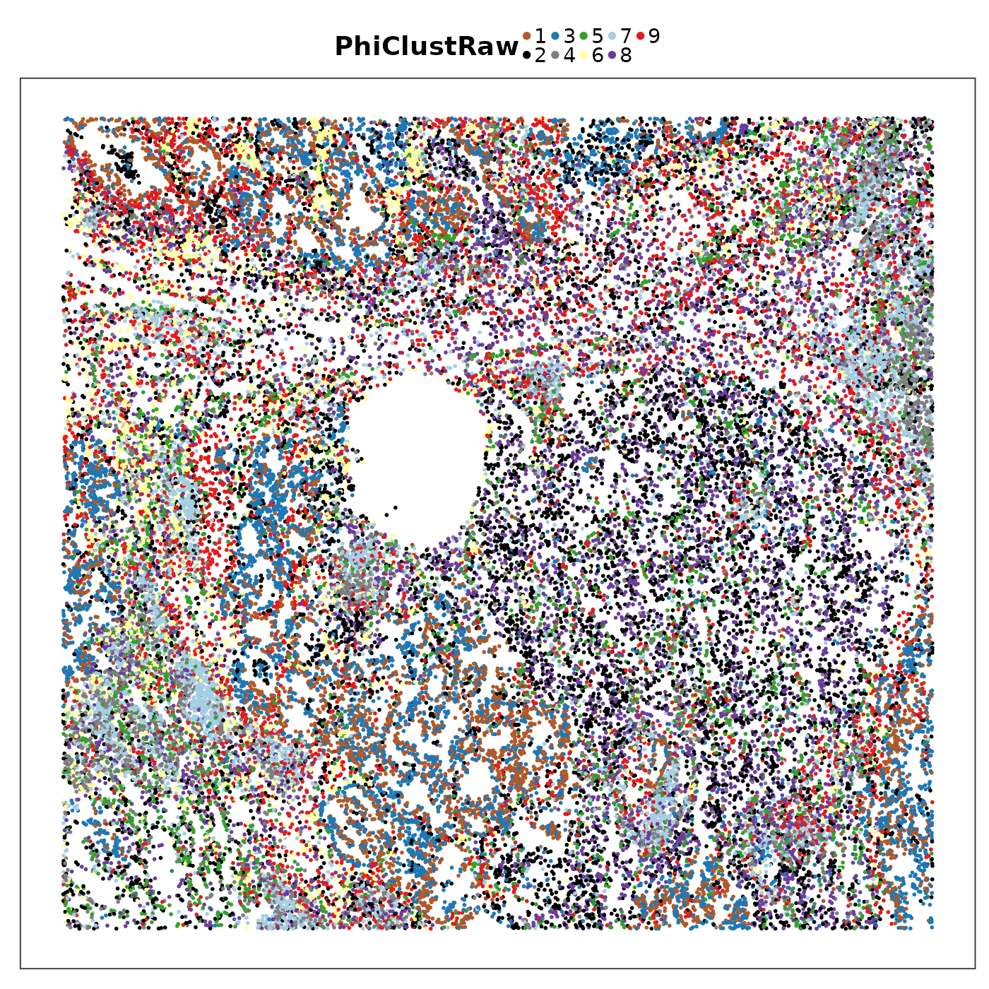
How is the PhiSpace k-means result compared to Banksy? Here we’re facing a common problem in visual comparison of clustering results, namely non-matching colour code. This is because the use of cluster labels is arbitrary, so even if our k-means and Banksy results both have number of clusters equal to 9, the labels from these two results do not correspond to each other.
It is possible to align cluster labels across clustering results
using algorithms from combinatorial optimisation.
PhiSpace::align_clusters does exactly that.
oldClust <- query$PhiClustRaw
refClust <- query$BanksyClust
newClust <- align_clusters(oldClust, refClust)
query$PhiClust_align <- newClust
Now visualise the aligned PhiSpace clusters.
VizSpatial(query,  groupBy = "PhiClust_align", ptSize = 1, legend.position = "top", legend.symb.size = 2) +
scale_colour_manual(values = tempClustCols) 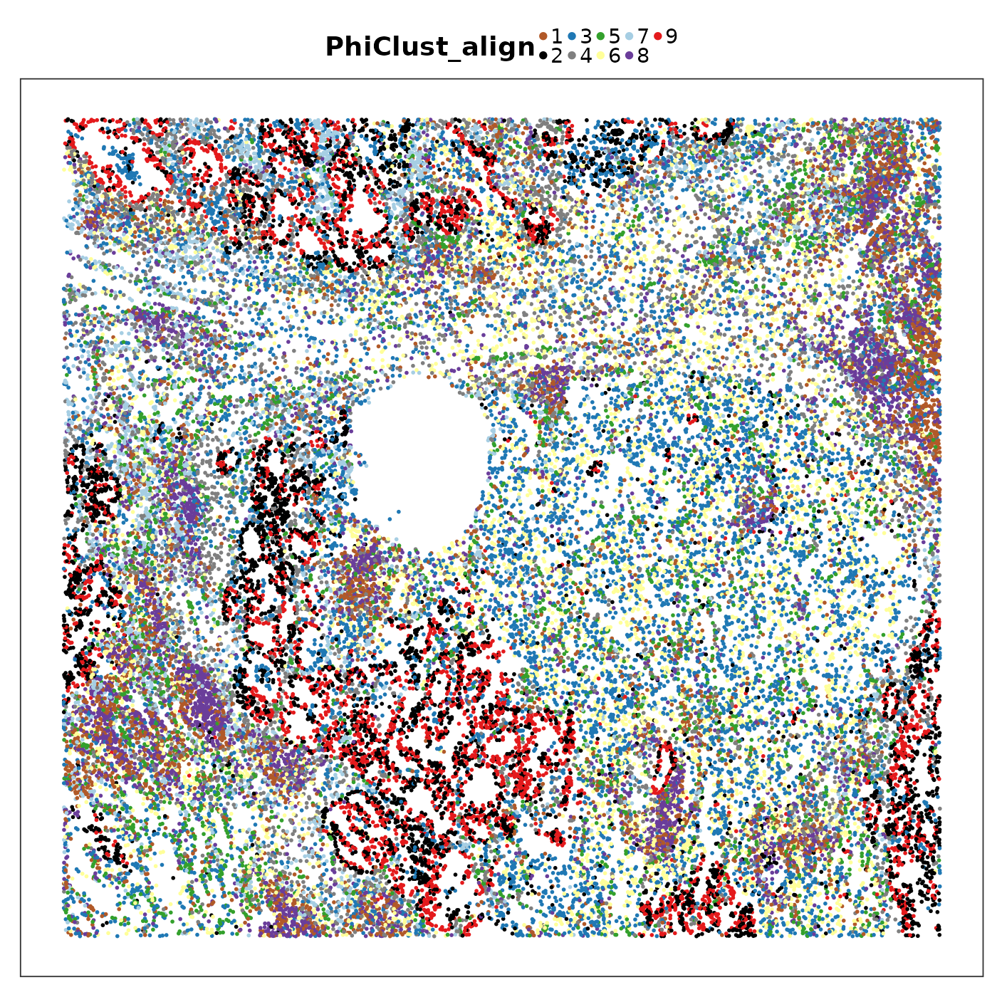
We can see that PhiSpace + k-means identified some similar niches as Banksy. But the niches seemed to lack spatial continuity. This can be improved if we do a spatial smoothing of PhiSpace scores before clustering.
Incorporate spatial information in PhiSpace scores
Spatial smoothing is a easy and flexible trick to increase spatial continuity of results. Bansky applied spatial smoothing to gene expression; here we apply it to PhiSpace scores.
query <- spatialSmoother(query, smoothReducedDim = T, kernel = "gaussian", k = 15)## Using spatial coordinates from SpatialExperiment object
## Smoothing reduced dimensions: PhiSpace
## Finding k-nearest neighbors...
## Computing kernel weights...
## Performing spatial smoothing...
## | | | 0% | | | 1% | |= | 1% | |= | 2% | |== | 2% | |== | 3% | |== | 4% | |=== | 4% | |=== | 5% | |==== | 5% | |==== | 6% | |===== | 6% | |===== | 7% | |===== | 8% | |====== | 8% | |====== | 9% | |======= | 9% | |======= | 10% | |======= | 11% | |======== | 11% | |======== | 12% | |========= | 12% | |========= | 13% | |========= | 14% | |========== | 14% | |========== | 15% | |=========== | 15% | |=========== | 16% | |============ | 16% | |============ | 17% | |============ | 18% | |============= | 18% | |============= | 19% | |============== | 19% | |============== | 20% | |============== | 21% | |=============== | 21% | |=============== | 22% | |================ | 22% | |================ | 23% | |================ | 24% | |================= | 24% | |================= | 25% | |================== | 25% | |================== | 26% | |=================== | 26% | |=================== | 27% | |=================== | 28% | |==================== | 28% | |==================== | 29% | |===================== | 29% | |===================== | 30% | |===================== | 31% | |====================== | 31% | |====================== | 32% | |======================= | 32% | |======================= | 33% | |======================= | 34% | |======================== | 34% | |======================== | 35% | |========================= | 35% | |========================= | 36% | |========================== | 36% | |========================== | 37% | |========================== | 38% | |=========================== | 38% | |=========================== | 39% | |============================ | 39% | |============================ | 40% | |============================ | 41% | |============================= | 41% | |============================= | 42% | |============================== | 42% | |============================== | 43% | |============================== | 44% | |=============================== | 44% | |=============================== | 45% | |================================ | 45% | |================================ | 46% | |================================= | 46% | |================================= | 47% | |================================= | 48% | |================================== | 48% | |================================== | 49% | |=================================== | 49% | |=================================== | 50% | |=================================== | 51% | |==================================== | 51% | |==================================== | 52% | |===================================== | 52% | |===================================== | 53% | |===================================== | 54% | |====================================== | 54% | |====================================== | 55% | |======================================= | 55% | |======================================= | 56% | |======================================== | 56% | |======================================== | 57% | |======================================== | 58% | |========================================= | 58% | |========================================= | 59% | |========================================== | 59% | |========================================== | 60% | |========================================== | 61% | |=========================================== | 61% | |=========================================== | 62% | |============================================ | 62% | |============================================ | 63% | |============================================ | 64% | |============================================= | 64% | |============================================= | 65% | |============================================== | 65% | |============================================== | 66% | |=============================================== | 66% | |=============================================== | 67% | |=============================================== | 68% | |================================================ | 68% | |================================================ | 69% | |================================================= | 69% | |================================================= | 70% | |================================================= | 71% | |================================================== | 71% | |================================================== | 72% | |=================================================== | 72% | |=================================================== | 73% | |=================================================== | 74% | |==================================================== | 74% | |==================================================== | 75% | |===================================================== | 75% | |===================================================== | 76% | |====================================================== | 76% | |====================================================== | 77% | |====================================================== | 78% | |======================================================= | 78% | |======================================================= | 79% | |======================================================== | 79% | |======================================================== | 80% | |======================================================== | 81% | |========================================================= | 81% | |========================================================= | 82% | |========================================================== | 82% | |========================================================== | 83% | |========================================================== | 84% | |=========================================================== | 84% | |=========================================================== | 85% | |============================================================ | 85% | |============================================================ | 86% | |============================================================= | 86% | |============================================================= | 87% | |============================================================= | 88% | |============================================================== | 88% | |============================================================== | 89% | |=============================================================== | 89% | |=============================================================== | 90% | |=============================================================== | 91% | |================================================================ | 91% | |================================================================ | 92% | |================================================================= | 92% | |================================================================= | 93% | |================================================================= | 94% | |================================================================== | 94% | |================================================================== | 95% | |=================================================================== | 95% | |=================================================================== | 96% | |==================================================================== | 96% | |==================================================================== | 97% | |==================================================================== | 98% | |===================================================================== | 98% | |===================================================================== | 99% | |======================================================================| 99% | |======================================================================| 100%
## Spatial smoothing completed!
## Added smoothed reduced dimension: PhiSpace_smoothedRun k-means again on spatially smoothed PhiSpace scores.
Lung5Rep1_PhiSmoothClusts <- clusterPhiSpace(query, k = 9, ncomp = 30, seed = 32123, reducedDimName = "PhiSpace_smoothed")
# save(Lung5Rep1_PhiSmoothClusts, file = "~/Dropbox/Research_projects/MIG_Spatial_Workshop/output/Lung5Rep1_PhiSmoothClusts.rda")
data("Lung5Rep1_PhiSmoothClusts")
PhiClust_smooth <- as.character(Lung5Rep1_PhiSmoothClusts$clusters)
# Align clusters
query$PhiClust <- align_clusters(PhiClust_smooth, query$BanksyClust)
VizSpatial(allTissues[["Lung5_Rep1"]], ptSize = 0.5, groupBy = "region", legend.position = "bottom", legend.symb.size = 2) 
VizSpatial(allTissues[["Lung5_Rep1"]], ptSize = 1, groupBy = "BanksyClust", legend.position = "bottom", legend.symb.size = 2) +
  scale_colour_manual(values = tempClustCols)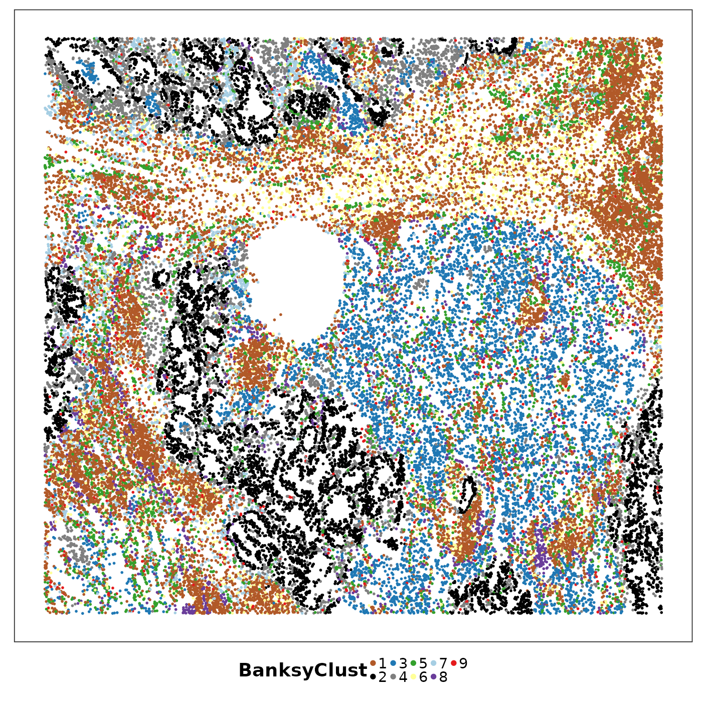
VizSpatial(query,  groupBy = "PhiClust", ptSize = 1, legend.position = "bottom", legend.symb.size = 2) +
scale_colour_manual(values = tempClustCols) 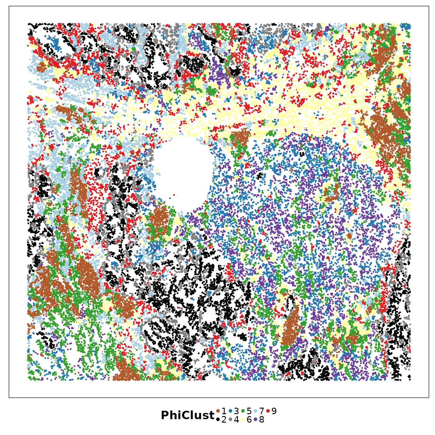
Look how a simple smoothing step has greatly enhanced the spatial continuity of PhiSpace niches. It seems both more biologically interpretable and more aesthetically appealing.
Alternatively, we can use hoodscanR, a package dedicated
to niche identification based on discrete or continuous cell type
annotation.
query$PhiCellType <- getClass(reducedDim(query, "PhiSpace"))
# find neighbouring cells using an approximate nearest neighbour search
set.seed(1000)
nb_cells = findNearCells(query, k = 100, anno_col = "PhiCellType")
nb_cells$cells[1:5, 1:5]
nb_cells$distance[1:5, 1:5]
probmat = scanHoods(nb_cells$distance)
dim(probmat)
# compute probability of each each cell type in the neighbour hood of each cell
PhiSpaceProb <- Score2Prob(reducedDim(query,"PhiSpace"))
# hoods <- mergeByGroup(probmat, PhiSpaceProb, continuousAnnotation = T)
# query <- mergeHoodSpe(query, hoods)
# query <- clustByHood(query, pm_cols = colnames(hoods), k = 9)
neighbourhoods <- hoodscanR::mergeByGroup(probmat, nb_cells$cells)
neighbourhoods[1:5, 1:5]
query <- mergeHoodSpe(query, neighbourhoods)
set.seed(1000)
query <- clustByHood(query, pm_cols = colnames(neighbourhoods), k = 9, val_name = "hsR_clusters")
# Align clusters
query$hsR_clusters <- align_clusters(query$hsR_clusters, query$BanksyClust)
VizSpatial(query,  groupBy = "hsR_clusters", ptSize = 1, legend.position = "bottom", legend.symb.size = 2) +
  scale_colour_manual(values = tempClustCols)
What are these niches?
The first thing we notice (ie I noticed) is that the tumour region was more finely clusters by PhiSpace compared to Banksy. Instead of the black–grey division as in Banksy, now we have this black–red–grey division. Note that the total number of clusters is the same in two cases. It seems that based on PhiSpace annotation we can identify more heterogeneity in the tumour region.
The second thing is that there were some interesting subclusters emerging in the stromal region. Notably the purple cluster became more prominant in PhiSpace result.
Let’s use PLS again to see what cell types are enriched in these newly identified niches.
featSelRes <- rankFeatures(query, "PhiClust", method = "PLSDA", ncomp = length(unique(query$PhiClust)))
selectFeat(featSelRes$importance_scores)$orderedFeatMat[1:5,]
## 1 2 3
## [1,] "B(luca)" "Mesothelial(mesen)" "Neutro(luca)"
## [2,] "CD4(immu)" "Tumour(luca)" "Sec_SCGB3A2(epi)"
## [3,] "B(immu)" "gCap(endo)" "Myeloid_Divid(luca)"
## [4,] "cDC1(immu)" "AT2/Club_Trans(luca)" "Sec_SCGB1A1/MUC5B(epi)"
## [5,] "Myeloid_Divid(luca)" "Basal(epi)" "Mono(luca)"
## 4 5 6
## [1,] "FB_PLIN2(mesen)" "Venule(endo)" "Mph_Interst(immu)"
## [2,] "Tumour(luca)" "Sec_SCGB1A1/MUC5B(epi)" "Mono_Inflam(immu)"
## [3,] "Plasma(luca)" "Pericyte(mesen)" "cDC2(immu)"
## [4,] "gCap(endo)" "CD4(immu)" "Pericyte(mesen)"
## [5,] "Mono_Inflam(immu)" "FB_Myo_Act(mesen)" "DC_Mono(immu)"
## 7 8 9
## [1,] "Plasma(luca)" "Mph(luca)" "FB_Myo_Act(mesen)"
## [2,] "Plasma_Divid(luca)" "Mph_Alv(luca)" "Stromal_Divid(luca)"
## [3,] "B(luca)" "Mph_Mono(immu)" "Mesothelial(mesen)"
## [4,] "Neutro(luca)" "Mono(luca)" "FB_Peribronch(luca)"
## [5,] "CD4(immu)" "CD4(luca)" "cDC2(luca)"Compare the three tumour niches, clusters 2 (black), 4 (gray) and 9 (red);
Cluster 8 (purple) is enriched by macrophages.
##            used  (Mb) gc trigger   (Mb)  max used  (Mb)
## Ncells  9680222 517.0   15940374  851.4  15940374 851.4
## Vcells 76645290 584.8  154443855 1178.4 128636546 981.5
Multi-sample analysis
PhiSpace is useful for multi-sample analysis, where we have a collection of tissue sections, consecutive or from different patients.
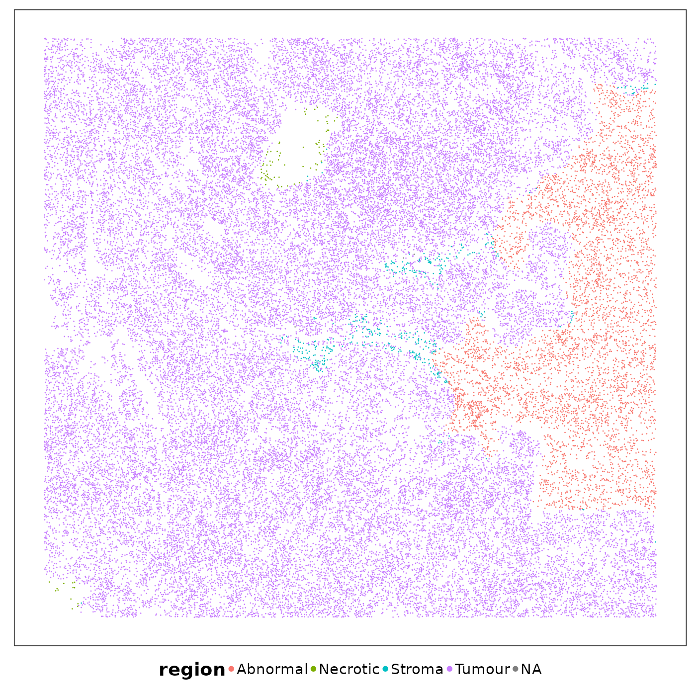
First let’s look at these tissues and the pathological annotation. They have very different compositions of niches.
lapply(1:length(allTissues), function(ii){
  p <- VizSpatial(
    allTissues[[ii]], ptSize = 0.5, groupBy = "region", legend.position = "bottom", legend.symb.size = 2
  )
  return(p)
})
Tumour heterogeneity
Apart from Lung6, which was from a LUSC patient, all remaining lung samples were from LUAD patients. PhiSpace scores can be used to examine the heterogeneity of lung tumours.
tumourNames <- c("Lung5_Rep1", "Lung5_Rep2", "Lung5_Rep3", "Lung6", "Lung9_Rep1", "Lung12", "Lung13")
tumourSig <- vector("list", length(tumourNames))
names(tumourSig) <- tumourNames
#Individual tumours
for(ii in 1:length(tumourNames)){
  tissueName <- tumourNames[ii]
  query <- allTissues[[tissueName]]
  query <- query[,!is.na(query$region)]
  regCoef <- rankFeatures(query, "region", ncomp = length(unique(query$region)))$importance_scores
  selectedPheno <- selectFeat(regCoef, nfeat = 5, absVal = F)
  tumourSig[[ii]] <- selectedPheno$orderedFeatMat[,"Tumour"]
}
## Warning in irlba(x, n, ...): You're computing too large a percentage of total
## singular values, use a standard svd instead.
## Warning in irlba(x, n, ...): You're computing too large a percentage of total
## singular values, use a standard svd instead.Only Lung6 tumour showed a strong presence of immune cells, including natural killers, neutrophils and CD4 T cells. Tumours in the three biological repeats from Lung5 (consecutive sections) had very similar cell states.
do.call(cbind, tumourSig)[1:10,]## Lung5_Rep1 Lung5_Rep2
## [1,] "Tumour(luca)" "Sec_SCGB1A1/MUC5B(epi)"
## [2,] "Sec_SCGB1A1/MUC5B(epi)" "Tumour(luca)"
## [3,] "AT2/Club_Trans(luca)" "AT2/Club_Trans(luca)"
## [4,] "Mesothelial(mesen)" "Sec_SCGB3A2(epi)"
## [5,] "Mph_Alv(immu)" "Mesothelial(mesen)"
## [6,] "AT2_Trans(epi)" "Basal(epi)"
## [7,] "KRT5-/KRT17+(epi)" "SMC(mesen)"
## [8,] "Basal(epi)" "Stromal_Divid(luca)"
## [9,] "Mesothelial(luca)" "FB_Adv(mesen)"
## [10,] "Sec_SCGB3A2(epi)" "FB_Myo_Act(mesen)"
## Lung5_Rep3 Lung6 Lung9_Rep1
## [1,] "Tumour(luca)" "Tumour(luca)" "Tumour(luca)"
## [2,] "Mesothelial(mesen)" "Neutro(luca)" "FB_Peribronch(luca)"
## [3,] "AT2/Club_Trans(luca)" "NK(immu)" "Stromal_Divid(luca)"
## [4,] "Sec_SCGB1A1/MUC5B(epi)" "FB_Myo_Act(mesen)" "FB_Myo_Act(mesen)"
## [5,] "Mph_Alv(immu)" "Stromal_Divid(luca)" "Plasma(immu)"
## [6,] "AT2_Trans(epi)" "Plasma(immu)" "Mph_Interst(immu)"
## [7,] "Basal(epi)" "Endo_Lymphatic(luca)" "Arteriole(endo)"
## [8,] "KRT5-/KRT17+(epi)" "SysVenous(endo)" "Epi_ROS1(luca)"
## [9,] "Mono(luca)" "FB_Adv(mesen)" "aCap(endo)"
## [10,] "Sec_SCGB3A2(epi)" "CD4(immu)" "CD4(immu)"
## Lung12 Lung13
## [1,] "AT1(luca)" "Mesothelial(mesen)"
## [2,] "Mesothelial(mesen)" "AT2/Club_Trans(luca)"
## [3,] "AT2/Club_Trans(luca)" "Tumour(luca)"
## [4,] "SysVenous(endo)" "Mph_Alv(immu)"
## [5,] "AT2_Trans(epi)" "AT2_Trans(epi)"
## [6,] "KRT5-/KRT17+(epi)" "Mesothelial(luca)"
## [7,] "Neutro(luca)" "KRT5-/KRT17+(epi)"
## [8,] "Ciliated_Diff(epi)" "AT1(luca)"
## [9,] "Mph_Alv(immu)" "Plasma(immu)"
## [10,] "Mono(luca)" "AT2(luca)"Niches across samples
We’ve seen that PhiSpace clustering revealed more fine-grained niches compared to pathological annotations. Can we identify niches across tissues, so that the same niche has the same cell states across tissue samples? Multi-sample niche identification based on gene expression is challenging since there might be batch effects between tissue slides. PhiSpace scores from multiple samples do not suffer from batch effects since they were obtained using the same references. Hence to obtain cross-sample niches we simply concatenate the PhiSpace scores of all tissues and then do a k-means clustering.
Run clustering.
allTissues <- lapply(
  allTissues, function(spe) spatialSmoother(spe, smoothReducedDim = T, kernel = "gaussian", k = 15, verbose = F)
)
mat2clust <- lapply(1:length(allTissues), function(x) reducedDim(allTissues[[x]], "PhiSpace_smoothed"))
mat2clust <- do.call(rbind, mat2clust)
multiClustRes <- clusterPhiSpace(mat2clust, k = 9, iter.max = 1000, seed = 83904)
# save(multiClustRes, file = "~/Dropbox/Research_projects/MIG_Spatial_Workshop/output/multiClustRes.rda")
Or load pre-computed clustering results.
data("multiClustRes")
for(ii in 1:length(allTissues)){
  spe <- allTissues[[ii]]
  spe$multiSampClust <- as.character(multiClustRes$clusters[colnames(spe)])
  allTissues[[ii]] <- spe
}
Visualise PhiSpace niches.
lapply(1:length(allTissues), function(ii){
  p <- VizSpatial(
    allTissues[[ii]], ptSize = 1, groupBy = "multiSampClust", legend.position = "bottom", legend.symb.size = 2
  ) + scale_colour_brewer(palette = "Set1")
  return(p)
})
## [[1]]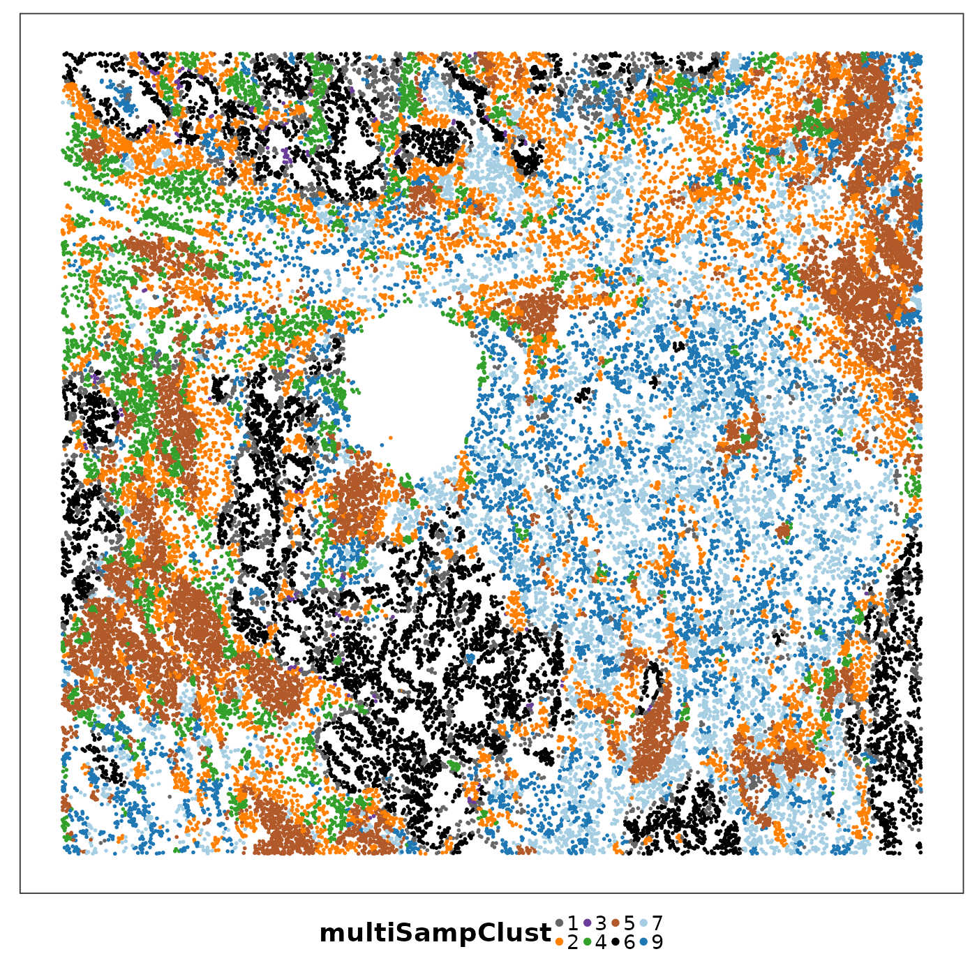
##
## [[2]]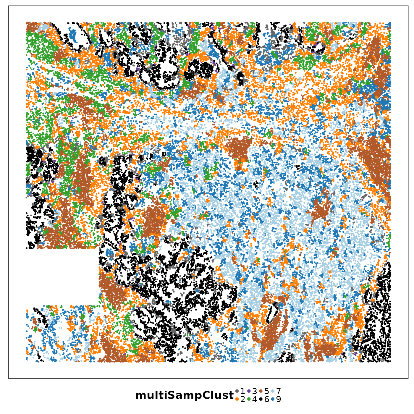
##
## [[3]]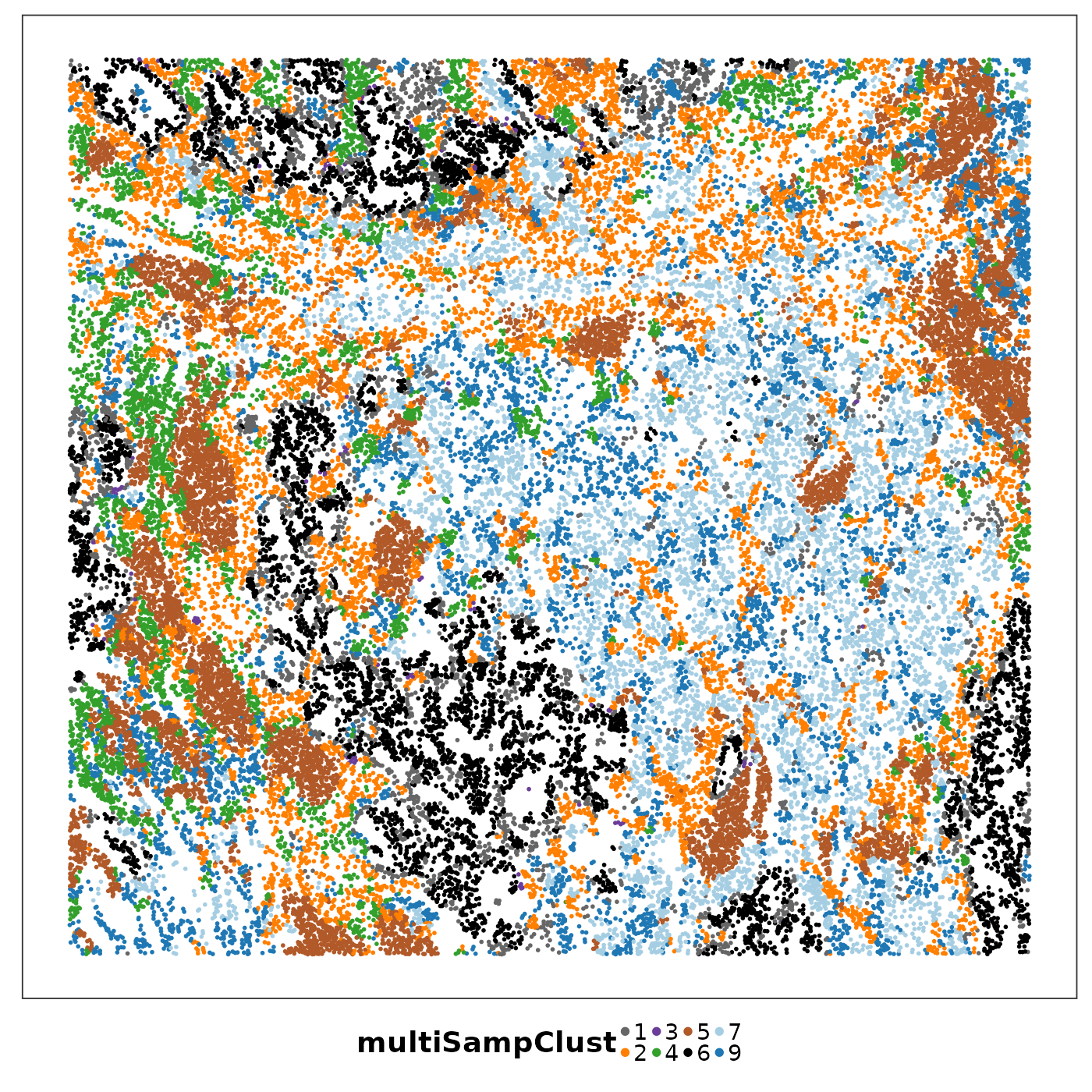
##
## [[4]]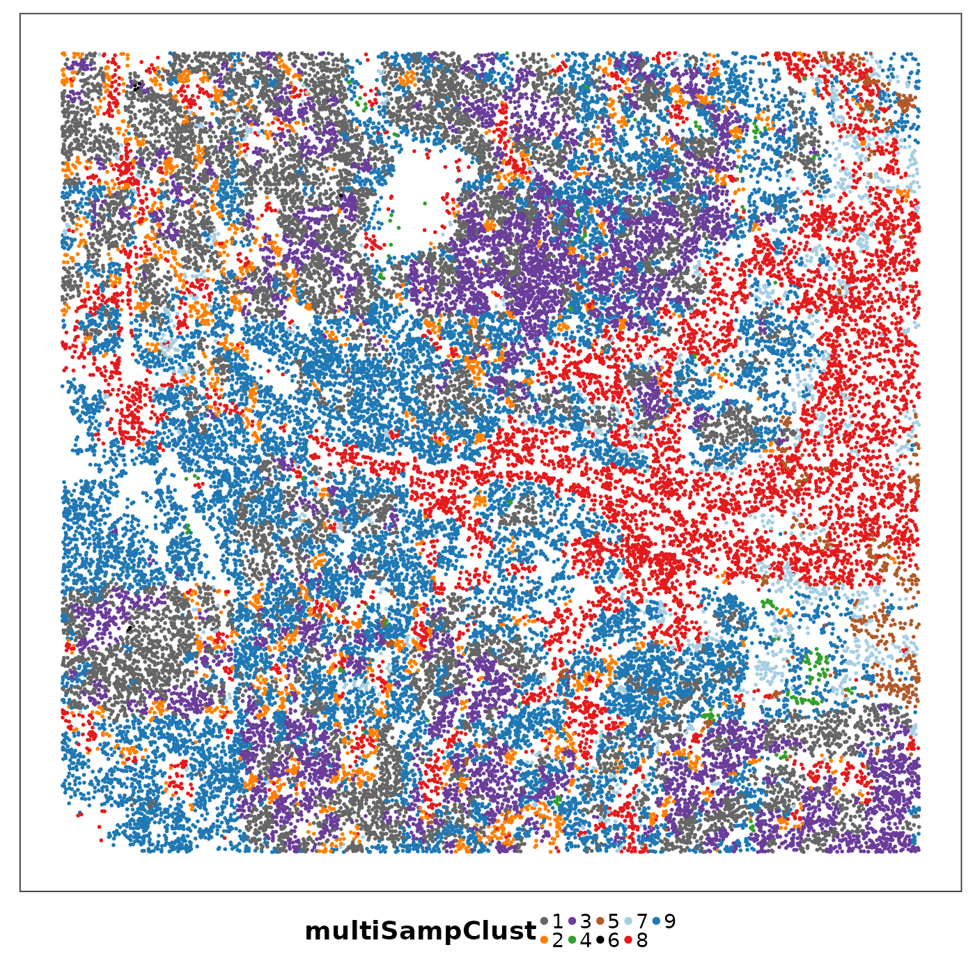
##
## [[5]]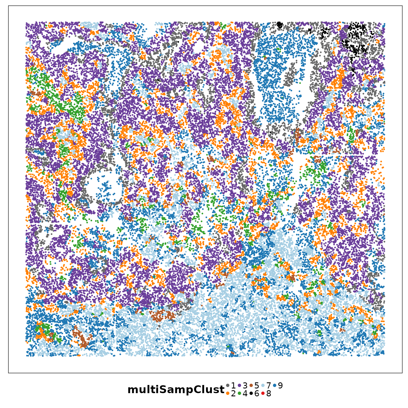
##
## [[6]]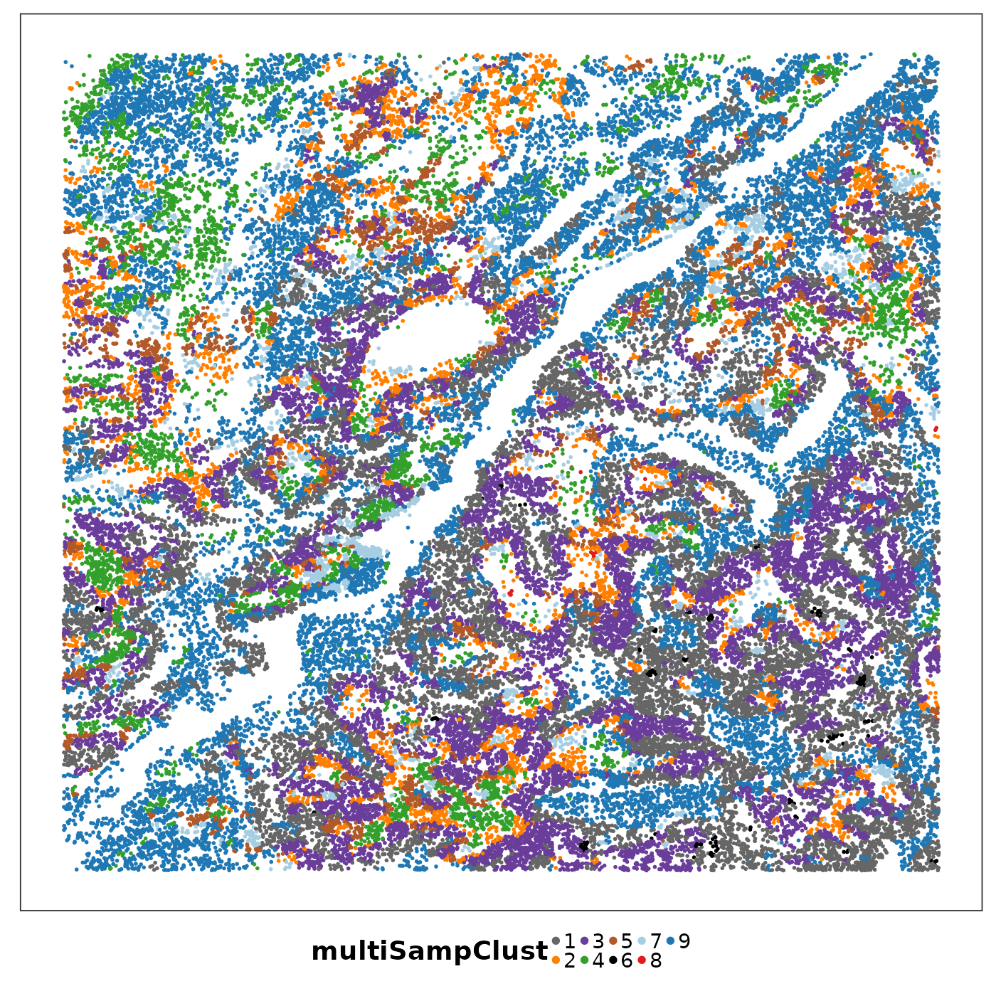
##
## [[7]]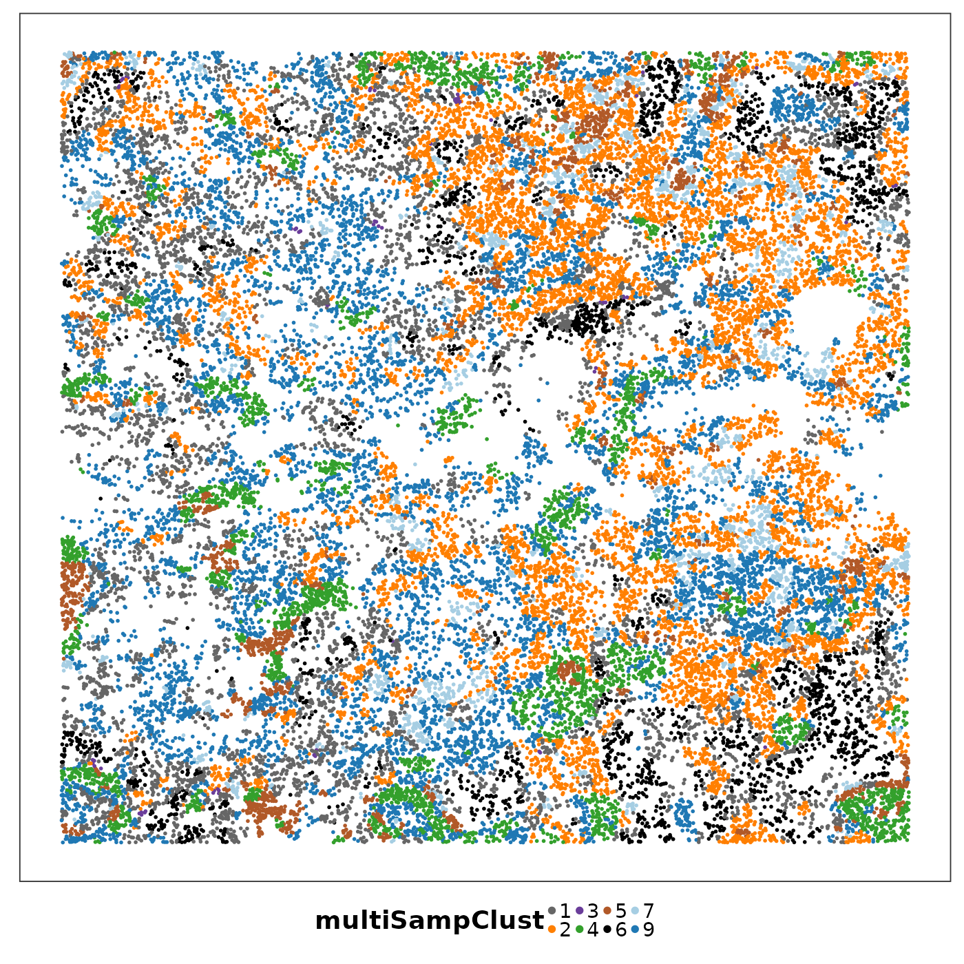
##
## [[8]]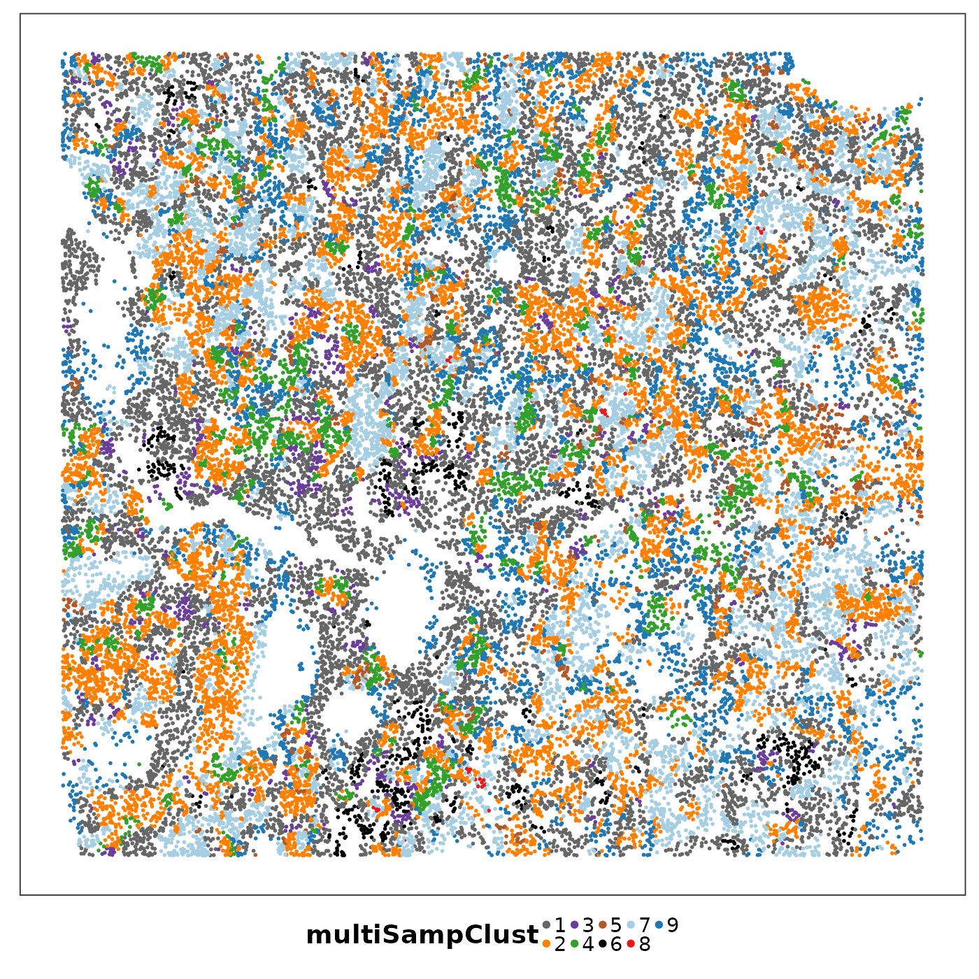
We can see that some niches only appeared in certain tissue sections. Let’s visualise the top enriched cell types in each of these niches.
df <- lapply(1:length(allTissues), function(x) reducedDim(allTissues[[x]], "PhiSpace"))
df <- do.call(rbind, df)
df <- as.data.frame(df) %>% mutate(cluster = as.character(multiClustRes$clusters))
plotGroups(
  df, "cluster", title = "Top 5 Cell Types per Cluster (Ordered by Median Score)",
  subtitle = "Boxplots show distribution of scores within each cluster"
)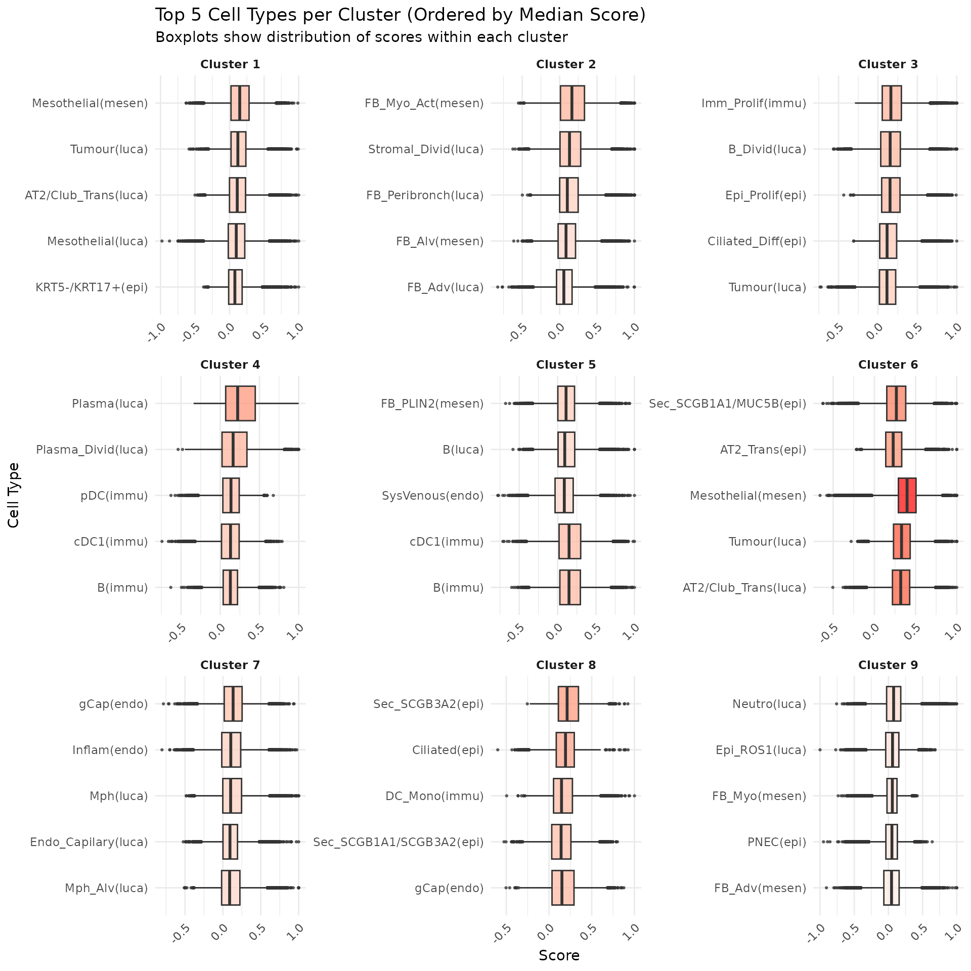
Cluster 8 (red) had a mixture of secretory, ciliated, capillary cells, with presence of monocyte-drived dendritic cells (indicating inflammation). This cluster was unique to lung6, and was annotated as abnormal stroma by the pathologist.
There were three clusters with strong tumour identity, cluster 1 (gray), cluster 3 (purple) and cluster 6 (black). Black was populous in lung5; gray and purple were more populous in other lungs.
What was annotated simply as ‘tumour’ by the pathologist now shows more heterogeneity after PhiSpace clustering.
Cell type co-presence
In a complex tissue environment, such as tumour microenvironment, cells often exhibit hybrid cell states. For example, we have seen that tumour cells can even simultaneously resemble cell types from different lineages. Another for this hybridity is due to technical reasons, such as imperfect cell segmentation and transcript diffusion. That is, cells may not be perfectly segmented, so that a segmented cell may actually contain transcripts from neighbouring cells. Transcript diffusion refers to the phenomenon that transcripts drift to different locations during the sequencing process, which is a common phenomenon in data from sequencing-based ST platforms (You et al., 2024).
With PhiSpace scores, we can look at cell type co-presence in each spatial unit. These co-presence patterns often have power to differentiate different niches from different tissue samples. As an example, we first compute the cell type co-presence matrices of different pathological niches in Lung5_Rep1. Here we only
tissueName <- "Lung5_Rep1"
PhiSc <- reducedDim(allTissues[[tissueName]], "PhiSpace")
# PhiSc <- PhiSc[,!grepl("(luca)", colnames(PhiSc))]
colDat <- colData(allTissues[[tissueName]])
coords <- spatialCoords(allTissues[[tissueName]])

table(colDat$region)

corMat <- cor(PhiSc[colDat$region=="Tumour",])
cVars <- colVars(corMat)
selectedTypes <- names(cVars)[rank(-cVars) <= 25]
corMat <- corMat[selectedTypes, selectedTypes]
plotCorrelation(corMat, seriation_method = "PCA")

corMat <- cor(PhiSc[colDat$region=="Stroma",])
cVars <- colVars(corMat)
selectedTypes <- names(cVars)[rank(-cVars) <= 25]
corMat <- corMat[selectedTypes, selectedTypes]
plotCorrelation(corMat, seriation_method = "PCA")

corMat <- cor(PhiSc[colDat$region=="Fibrotic",])
cVars <- colVars(corMat)
selectedTypes <- names(cVars)[rank(-cVars) <= 25]
corMat <- corMat[selectedTypes, selectedTypes]
plotCorrelation(corMat, seriation_method = "PCA")
Generate niche-specific co-localisation matrices for all tissue samples. How do we analyse this many matrices? An easy approach is to vectorise them and then do PCA.
nicheVarName <- "multiSampClust"
corMatVec <- lapply(
  1:length(tissueNames_CosMx),
  function(ii){
    # For each tissue
    tissueName <- tissueNames_CosMx[ii]
    query <- allTissues[[tissueName]]
    sc <- reducedDim(query, "PhiSpace")
    # sc <- sc[,colnames(sc)[grepl("(luca)", colnames(sc))]]
    # colnames(sc) <- gsub("\\([^)]*\\)", "", colnames(sc))
    reducedDim(query, "PhiSpace") <- sc
    niches <- colData(query)[,nicheVarName]
    tempNicheNames <- unique(niches)
    # List of correlation matrices (corMats)
    corMat_list <- lapply(
      tempNicheNames,
      function(x){
        nicheName <- x
        corMat <- cor(reducedDim(query[,niches==nicheName], "PhiSpace"))
        return(corMat)
      }
    )
    names(corMat_list) <- tempNicheNames
    # Labels for entries in each corMat
    cTypeCombo <- outer(
          rownames(corMat_list[[1]]), colnames(corMat_list[[1]]),
          function(x, y) paste0(x, "<->", y)
        )

    # Vectorise corMats
    corMatVec <- sapply(
      corMat_list,
      function(x) as.vector(x[lower.tri(x)])
    ) %>%
      `colnames<-`(
        paste0(tempNicheNames, "_", tissueName)
      ) %>%
      `rownames<-`(
        cTypeCombo[lower.tri(cTypeCombo)]
      ) %>% t()
    corMatVec <- corMatVec %>%
      as.data.frame() %>%
      mutate(
        niche = tempNicheNames,
        sample = rep(tissueName, nrow(corMatVec))
      )
    return(corMatVec)
  }
)
corMatVec <- do.call(rbind, corMatVec)

# Delete niches with fewer than 50 cells
minNicheCells <- 50
nicheTabs <- lapply(
  1:length(allTissues),
  function(x){
    tissueName <- names(allTissues)[x]
    out <- table(colData(allTissues[[x]])[,nicheVarName])
    names(out) <- paste0(names(out), "_", tissueName)
    return(out)
  }
)
nPerNiche <- do.call("c", nicheTabs)
corMatVec <- corMatVec[names(nPerNiche)[nPerNiche >= minNicheCells], ]

# PCA of vectorised matrices
set.seed(12361)
pca_res <- getPC(corMatVec %>% select(!c(niche, sample)) %>% as.matrix(), ncomp = 5)
Visualise the first two PCs and their loadings. It’s interesting to see how the three cancer niches were separated from other niches, and how both PCs contributed to this separation. Also we noticed that cancer niches from the same tissue sample tended to cluster together. This suggests that, though the same niche across different tissues was defined by the same cell states, it had very different co-presence patterns across tissues. That is, cell type co-presence tells us something that’s not in the cell type score.
df <- as.data.frame(pca_res$scores)
df$sampIDs <- gsub("^[^_]*_", "", rownames(df))
df$niche <- corMatVec$niche
ggplot(df, aes(x = comp1, y = comp2, colour = niche)) +
  geom_text(aes(label = sampIDs)) +
  theme_bw() + scale_colour_brewer(palette = "Set1") + xlim(-6.5, 7)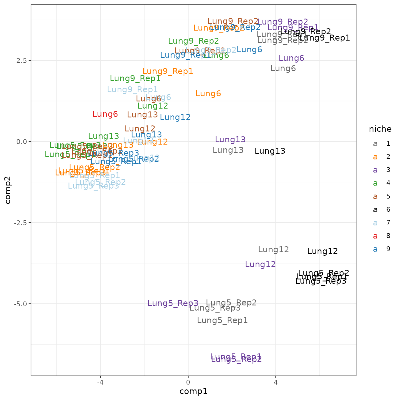
# Loading# Loadingniche
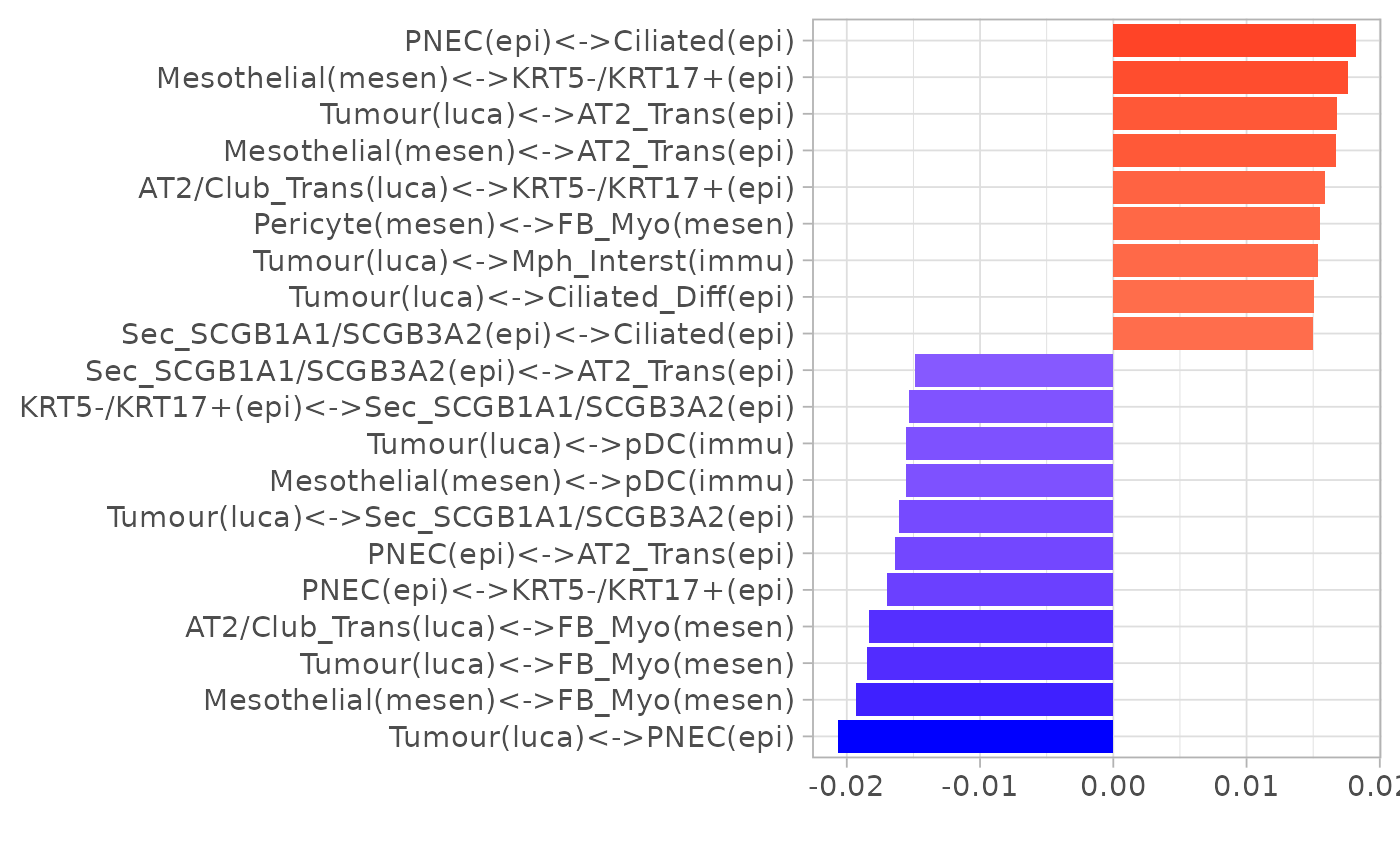
plotLoadings(pca_res$loadings, "comp1", showNeg = F, absVal = T, nfeat = 10)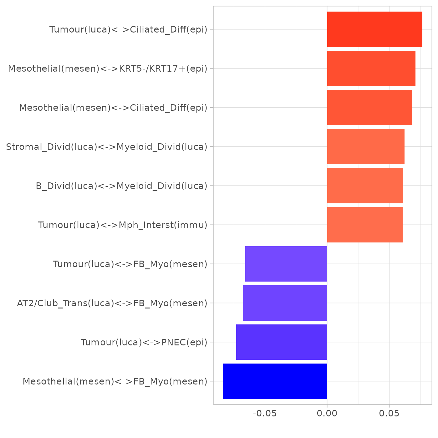
plotLoadings(pca_res$loadings, "comp2", showNeg = F, absVal = T, nfeat = 10)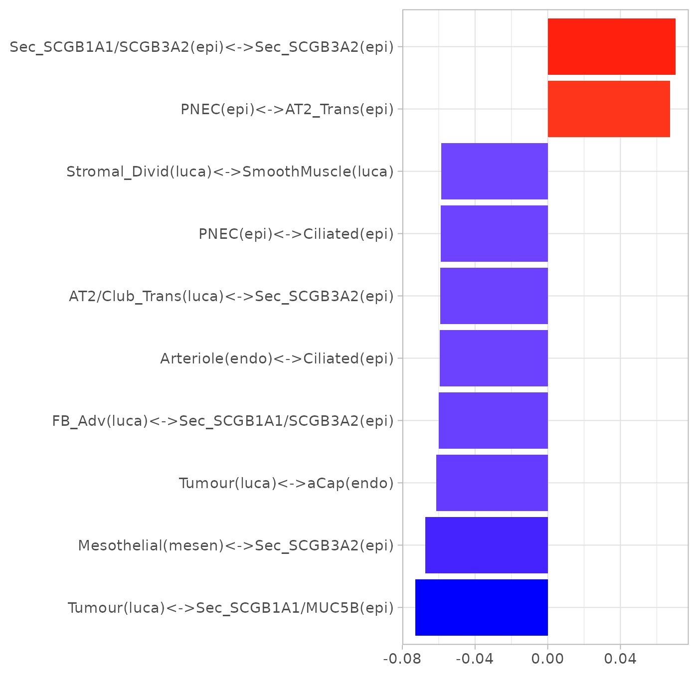
Note: PNEC stands for pulmonary neuroendocrine cell.
Neither PC1 or PC2 perfectly separated cancer from non-cancer niches. Next we use an interpretable classification algorithm DWD to separate them and visualise the loadings.
suppressPackageStartupMessages(library(kerndwd))
# Binarise niches
nicheBinary <- as.numeric(corMatVec$niche %in% c("1", "3", "6"))
nicheBinary[nicheBinary == 0] <- -1
nicheBinaryByName <- rep("Non-cancer niches", length(nicheBinary))
nicheBinaryByName[nicheBinary == 1] <- "Cancer niches"
X = corMatVec %>% select(!c(niche, sample)) %>% as.matrix

dwd_res <- rankFeatures(X, response = nicheBinary, method = "DWD")
The idea of DWD is the find the best one dimension representation of the high dimensional data points that best separated the two classes (in this case, cancer and non-cancer niches).
dwd_res$scores %>% as.data.frame() %>% mutate(niche = nicheBinaryByName) %>%
  ggplot() + geom_density(aes(DWD_score, fill = niche), alpha = 0.5) +
  theme_bw() + theme(legend.title = element_text(face ="bold")) + xlab("DWD score")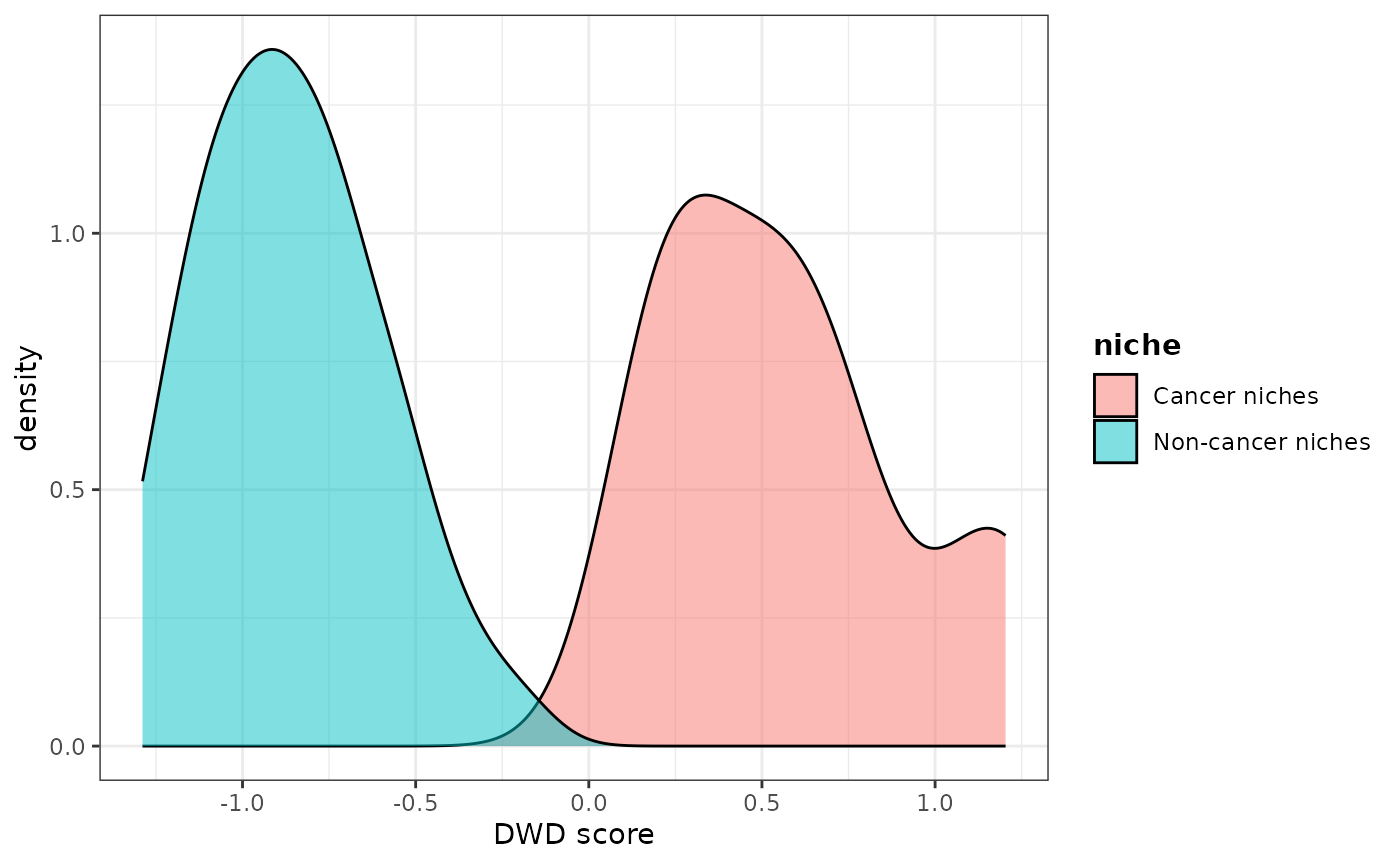
plotLoadings(dwd_res$importance_scores, "DWD_weight", nfeat = 20)